K-近邻和神经网络

K-近邻（K-NN, K-Nearest Neighbors）

原理

K-近邻（K-NN）是一种非参数分类和回归算法。K-NN 的主要思想是根据距离度量（如欧氏距离）找到训练数据集中与待预测样本最近的 K 个样本，并根据这 K 个样本的标签来进行预测。对于分类任务，K-NN 通过投票的方式选择出现最多的类别作为预测结果；对于回归任务，K-NN 通过计算 K 个最近邻样本的平均值来进行预测。

公式

K-NN 的主要步骤包括：

计算待预测样本与训练集中每个样本之间的距离。常用的距离度量包括欧氏距离、曼哈顿距离等。
找到距离最近的 K 个样本。
对于分类任务，通过投票决定预测结果：

其中，Nk 表示样本 x 的 K 个最近邻样本集合，I 是指示函数。

对于回归任务，通过计算平均值决定预测结果：

生活场景应用的案例

手写数字识别：K-NN 可以用于手写数字识别任务。假设我们有一个手写数字的图片数据集，每张图片都被标注了对应的数字。我们可以使用 K-NN 模型来识别新图片中的数字。

案例描述

假设我们有一个手写数字图片的数据集，包括以下特征：

图片像素值（每张图片由一个固定大小的像素矩阵表示）

我们希望通过这些像素值来预测图片中的数字。我们可以使用 K-NN 模型进行训练和预测。训练完成后，我们可以使用模型来识别新图片中的数字，并评估模型的性能。

代码解析

下面是一个使用 Python 实现上述手写数字识别案例的示例，使用了 scikit-learn 库。

import numpy as np
import pandas as pd
from sklearn.model_selection import train_test_split
from sklearn.neighbors import KNeighborsClassifier
from sklearn.metrics import accuracy_score, confusion_matrix, classification_report
import matplotlib.pyplot as plt
from sklearn.datasets import load_digits

# 载入手写数字数据集
digits = load_digits()
X = digits.data
y = digits.target

# 拆分训练集和测试集
X_train, X_test, y_train, y_test = train_test_split(X, y, test_size=0.2, random_state=42)

# 创建K-NN模型并训练
k = 5
model = KNeighborsClassifier(n_neighbors=k)
model.fit(X_train, y_train)

# 预测
y_pred = model.predict(X_test)

# 评估模型
accuracy = accuracy_score(y_test, y_pred)
cm = confusion_matrix(y_test, y_pred)
report = classification_report(y_test, y_pred)

print(f"Accuracy: {accuracy}")
print("Confusion Matrix:")
print(cm)
print("Classification Report:")
print(report)

# 可视化部分测试结果
fig, axes = plt.subplots(1, 5, figsize=(10, 3))
for ax, image, prediction in zip(axes, X_test, y_pred):
    ax.set_axis_off()
    image = image.reshape(8, 8)
    ax.imshow(image, cmap=plt.cm.gray_r, interpolation='nearest')
    ax.set_title(f'Pred: {prediction}')
plt.show()

在这个示例中：

我们使用了 sklearn.datasets 中的手写数字数据集。这个数据集包含了 8x8 像素的图片，每张图片代表一个手写数字。
将数据集拆分为训练集和测试集。
使用训练集训练 K-NN 分类模型。
通过测试集进行预测并评估模型的性能。
输出准确率（accuracy）、混淆矩阵（confusion matrix）和分类报告（classification report）。
可视化部分测试结果，展示模型的预测效果。

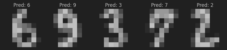
这个案例展示了如何使用 K-NN 模型来识别手写数字，基于图片的像素值特征。模型训练完成后，可以用于预测新图片中的数字，并帮助解决实际的手写数字识别问题。

神经网络（Neural Network）

原理

神经网络是一种模仿生物神经元结构的计算模型，由多个节点（神经元）和连接（权重）组成。神经网络主要由输入层、隐藏层和输出层构成，每一层包含若干神经元。通过层与层之间的连接和激活函数（如ReLU、Sigmoid等），神经网络能够拟合复杂的非线性关系，实现分类、回归等任务。

训练神经网络的过程通常使用反向传播算法，通过计算损失函数的梯度来调整网络的权重，以最小化预测误差。

公式

神经元的线性组合：

其中，xi 是输入，wi 是权重，b 是偏置，z 是神经元的加权和。

激活函数：常用的激活函数包括：

Sigmoid 函数：

ReLU 函数：

反向传播：

反向传播算法通过计算损失函数的梯度来更新权重：

其中，η 是学习率，L 是损失函数。

生活场景应用的案例

图像分类：神经网络广泛应用于图像分类任务。假设我们有一个包含手写数字图片的数据集，每张图片都被标注了对应的数字。我们可以使用神经网络模型来识别新图片中的数字。

案例描述

假设我们有一个手写数字图片的数据集，包括以下特征：

图片像素值（每张图片由一个固定大小的像素矩阵表示）

我们希望通过这些像素值来预测图片中的数字。我们可以使用神经网络模型进行训练和预测。训练完成后，我们可以使用模型来识别新图片中的数字，并评估模型的性能。

代码解析

下面是一个使用 Python 实现上述手写数字识别案例的示例，使用了 tensorflow 和 keras 库。

import numpy as np
import pandas as pd
from sklearn.model_selection import train_test_split
from sklearn.metrics import classification_report
import matplotlib.pyplot as plt
import tensorflow as tf
from tensorflow.keras.models import Sequential
from tensorflow.keras.layers import Dense, Flatten
from tensorflow.keras.utils import to_categorical
from sklearn.datasets import load_digits

# 载入手写数字数据集
digits = load_digits()
X = digits.images
y = digits.target

# 预处理数据
X = X / 16.0  # 将像素值归一化到 [0, 1]
y = to_categorical(y, num_classes=10)  # 将标签转换为one-hot编码

# 调整数据维度以适应TensorFlow模型
X = X.reshape(-1, 8, 8, 1)  # 使用-1使reshape自动计算样本数量

# 拆分训练集和测试集
X_train, X_test, y_train, y_test = train_test_split(X, y, test_size=0.2, random_state=42)

# 创建神经网络模型
model = Sequential([
    Flatten(input_shape=(8, 8, 1)),  # 展平输入图像
    Dense(128, activation='relu'),  # 隐藏层，包含128个神经元
    Dense(64, activation='relu'),  # 隐藏层，包含64个神经元
    Dense(10, activation='softmax')  # 输出层，包含10个神经元，对应10个类别
])

# 编译模型
model.compile(optimizer='adam', loss='categorical_crossentropy', metrics=['accuracy'])

# 训练模型
model.fit(X_train, y_train, epochs=20, batch_size=32, validation_split=0.2)

# 评估模型
loss, accuracy = model.evaluate(X_test, y_test)
y_pred = model.predict(X_test)
y_pred_classes = np.argmax(y_pred, axis=1)
y_true = np.argmax(y_test, axis=1)

print(f"Accuracy: {accuracy}")
print("Classification Report:")
print(classification_report(y_true, y_pred_classes))

# 可视化部分测试结果
fig, axes = plt.subplots(1, 5, figsize=(10, 3))
for ax, image, prediction in zip(axes, X_test, y_pred_classes):
    ax.set_axis_off()
    image = image.reshape(8, 8)  # 确保图像形状正确
    ax.imshow(image, cmap=plt.cm.gray_r, interpolation='nearest')
    ax.set_title(f'Pred: {prediction}')
plt.show()

在这个示例中：

我们使用了 sklearn.datasets 中的手写数字数据集。这个数据集包含了 8x8 像素的图片，每张图片代表一个手写数字。
将数据集拆分为训练集和测试集，并对数据进行预处理，将像素值归一化并将标签转换为 one-hot 编码。
创建了一个包含两个隐藏层的神经网络模型。
使用训练集训练神经网络模型。
通过测试集进行预测并评估模型的性能。
输出准确率（accuracy）和分类报告（classification report）。
可视化部分测试结果，展示模型的预测效果。

这个案例展示了如何使用神经网络模型来识别手写数字，基于图片的像素值特征。模型训练完成后，可以用于预测新图片中的数字，并帮助解决实际的手写数字识别问题。

具体应用

对预测结果进行可视化展示：

- 在预测结果后，展示原始图片及其预测结果。

保存和加载训练好的模型：

- 保存训练好的模型。
- 加载已保存的模型进行预测。

import os
import numpy as np
import pandas as pd
from sklearn.model_selection import train_test_split
from sklearn.metrics import classification_report
import matplotlib.pyplot as plt
import tensorflow as tf
from tensorflow.keras.models import Sequential, load_model
from tensorflow.keras.layers import Dense, Flatten
from tensorflow.keras.utils import to_categorical
from sklearn.datasets import load_digits
from PIL import Image  # 用于加载自定义图片

# 载入手写数字数据集
digits = load_digits()
X = digits.images
y = digits.target

# 预处理数据
X = X / 16.0  # 将像素值归一化到 [0, 1]
y = to_categorical(y, num_classes=10)  # 将标签转换为one-hot编码

# 调整数据维度以适应TensorFlow模型
X = X.reshape(-1, 8, 8, 1)  # 使用-1使reshape自动计算样本数量

# 拆分训练集和测试集
X_train, X_test, y_train, y_test = train_test_split(X, y, test_size=0.2, random_state=42)

# 创建神经网络模型
model = Sequential([
    Flatten(input_shape=(8, 8, 1)),  # 展平输入图像
    Dense(128, activation='relu'),  # 隐藏层，包含128个神经元
    Dense(64, activation='relu'),  # 隐藏层，包含64个神经元
    Dense(10, activation='softmax')  # 输出层，包含10个神经元，对应10个类别
])

# 编译模型
model.compile(optimizer='adam', loss='categorical_crossentropy', metrics=['accuracy'])

# 训练模型
model.fit(X_train, y_train, epochs=20, batch_size=32, validation_split=0.2)

# 保存训练好的模型
model.save('digit_recognition_model.h5')

# 加载训练好的模型
# model = load_model('digit_recognition_model.h5')

# 评估模型
loss, accuracy = model.evaluate(X_test, y_test)
y_pred = model.predict(X_test)
y_pred_classes = np.argmax(y_pred, axis=1)
y_true = np.argmax(y_test, axis=1)

print(f"Accuracy: {accuracy}")
print("Classification Report:")
print(classification_report(y_true, y_pred_classes))

# 可视化部分测试结果
fig, axes = plt.subplots(1, 5, figsize=(10, 3))
for ax, image, prediction in zip(axes, X_test, y_pred_classes):
    ax.set_axis_off()
    image = image.reshape(8, 8)  # 确保图像形状正确
    ax.imshow(image, cmap=plt.cm.gray_r, interpolation='nearest')
    ax.set_title(f'Pred: {prediction}')
plt.show()

# 加载并预处理单张图片
def load_and_preprocess_image(filepath):
    img = Image.open(filepath).convert('L')  # 转换为灰度图像
    img = img.resize((8, 8))  # 调整图像大小为8x8
    img = np.array(img) / 16.0  # 归一化像素值
    img = img.reshape(1, 8, 8, 1)  # 调整图像维度
    return img

# 加载并预处理文件夹中的所有图片
def load_images_from_folder(folder):
    images = []
    filepaths = []
    for filename in os.listdir(folder):
        if filename.endswith(('png', 'jpg', 'jpeg')):
            filepath = os.path.join(folder, filename)
            img = load_and_preprocess_image(filepath)
            images.append(img)
            filepaths.append(filepath)
    return np.vstack(images), filepaths

# 使用模型预测文件夹中的多张图片
def predict_custom_images_from_folder(folder):
    imgs, filepaths = load_images_from_folder(folder)
    preds = model.predict(imgs)
    pred_classes = np.argmax(preds, axis=1)
    return pred_classes, filepaths

# 示例：预测文件夹中的多张自定义图片并展示结果
custom_image_folder = 'path/to/your/folder'  # 替换为自定义图片文件夹路径
predicted_classes, filepaths = predict_custom_images_from_folder(custom_image_folder)

# 打印预测结果并可视化
fig, axes = plt.subplots(1, len(filepaths), figsize=(15, 3))
for ax, filepath, pred_class in zip(axes, filepaths, predicted_classes):
    ax.set_axis_off()
    img = Image.open(filepath).convert('L')
    img = img.resize((8, 8))
    img = np.array(img
    ax.imshow(img, cmap=plt.cm.gray_r, interpolation='nearest')
    ax.set_title(f'Pred: {pred_class}')
    print(f'The predicted class for {filepath} is: {pred_class}')
plt.show()

a. 添加更多的训练数据来提高模型的准确性。

b. 使用混淆矩阵来详细分析模型的分类结果。

import os
import numpy as np
import pandas as pd
from sklearn.model_selection import train_test_split
from sklearn.metrics import classification_report, confusion_matrix, ConfusionMatrixDisplay
import matplotlib.pyplot as plt
import tensorflow as tf
from tensorflow.keras.models import Sequential, load_model
from tensorflow.keras.layers import Dense, Flatten
from tensorflow.keras.utils import to_categorical
from tensorflow.keras.preprocessing.image import ImageDataGenerator
from sklearn.datasets import load_digits
from PIL import Image

# 载入手写数字数据集
digits = load_digits()
X = digits.images
y = digits.target

# 预处理数据
X = X / 16.0  # 将像素值归一化到 [0, 1]
y = to_categorical(y, num_classes=10)  # 将标签转换为one-hot编码

# 调整数据维度以适应TensorFlow模型
X = X.reshape(-1, 8, 8, 1)  # 使用-1使reshape自动计算样本数量

# 拆分训练集和测试集
X_train, X_test, y_train, y_test = train_test_split(X, y, test_size=0.2, random_state=42)

# 再拆分训练集以创建验证集
X_train, X_val, y_train, y_val = train_test_split(X_train, y_train, test_size=0.2, random_state=42)

# 数据扩充
datagen = ImageDataGenerator(
    rotation_range=10,
    zoom_range=0.1,
    width_shift_range=0.1,
    height_shift_range=0.1
)
datagen.fit(X_train)

# 创建神经网络模型
model = Sequential([
    Flatten(input_shape=(8, 8, 1)),  # 展平输入图像
    Dense(128, activation='relu'),  # 隐藏层，包含128个神经元
    Dense(64, activation='relu'),  # 隐藏层，包含64个神经元
    Dense(10, activation='softmax')  # 输出层，包含10个神经元，对应10个类别
])

# 编译模型
model.compile(optimizer='adam', loss='categorical_crossentropy', metrics=['accuracy'])

# 训练模型
model.fit(datagen.flow(X_train, y_train, batch_size=32), epochs=20, validation_data=(X_val, y_val))

# 保存训练好的模型
model.save('digit_recognition_model.h5')

# 加载训练好的模型
# model = load_model('digit_recognition_model.h5')

# 评估模型
loss, accuracy = model.evaluate(X_test, y_test)
y_pred = model.predict(X_test)
y_pred_classes = np.argmax(y_pred, axis=1)
y_true = np.argmax(y_test, axis=1)

print(f"Accuracy: {accuracy}")
print("Classification Report:")
print(classification_report(y_true, y_pred_classes))

# 生成混淆矩阵
cm = confusion_matrix(y_true, y_pred_classes)
disp = ConfusionMatrixDisplay(confusion_matrix=cm, display_labels=np.arange(10))
disp.plot(cmap=plt.cm.Blues)
plt.show()

# 可视化部分测试结果
fig, axes = plt.subplots(1, 5, figsize=(10, 3))
for ax, image, prediction in zip(axes, X_test, y_pred_classes):
    ax.set_axis_off()
    image = image.reshape(8, 8)  # 确保图像形状正确
    ax.imshow(image, cmap=plt.cm.gray_r, interpolation='nearest')
    ax.set_title(f'Pred: {prediction}')
plt.show()

# 加载并预处理单张图片
def load_and_preprocess_image(filepath):
    img = Image.open(filepath).convert('L')  # 转换为灰度图像
    img = img.resize((8, 8))  # 调整图像大小为8x8
    img = np.array(img) / 16.0  # 归一化像素值
    img = img.reshape(1, 8, 8, 1)  # 调整图像维度
    return img

# 加载并预处理文件夹中的所有图片
def load_images_from_folder(folder):
    images = []
    filepaths = []
    for filename in os.listdir(folder):
        if filename.endswith(('png', 'jpg', 'jpeg')):
            filepath = os.path.join(folder, filename)
            img = load_and_preprocess_image(filepath)
            images.append(img)
            filepaths.append(filepath)
    return np.vstack(images), filepaths

# 使用模型预测文件夹中的多张图片
def predict_custom_images_from_folder(folder):
    imgs, filepaths = load_images_from_folder(folder)
    preds = model.predict(imgs)
    pred_classes = np.argmax(preds, axis=1)
    return pred_classes, filepaths

# 示例：预测文件夹中的多张自定义图片并展示结果
custom_image_folder = 'path/to/your/folder'  # 替换为自定义图片文件夹路径
predicted_classes, filepaths = predict_custom_images_from_folder(custom_image_folder)

# 打印预测结果并可视化
fig, axes = plt.subplots(1, len(filepaths), figsize=(15, 3))
for ax, filepath, pred_class in zip(axes, filepaths, predicted_classes):
    ax.set_axis_off()
    img = Image.open(filepath).convert('L')
    img = img.resize((8, 8))
    img = np.array(img)
    ax.imshow(img, cmap=plt.cm.gray_r, interpolation='nearest')
    ax.set_title(f'Pred: {pred_class}')
    print(f'The predicted class for {filepath} is: {pred_class}')
plt.show()

a. 使用更多的手写数字样本进行训练，以提高模型对手写数字的识别能力。

b. 尝试使用不同的模型架构，如卷积神经网络（CNN），以提高模型的识别准确率。

import os
import numpy as np
import pandas as pd
from sklearn.model_selection import train_test_split
from sklearn.metrics import classification_report, confusion_matrix, ConfusionMatrixDisplay
import matplotlib.pyplot as plt
import tensorflow as tf
from tensorflow.keras.models import Sequential, load_model
from tensorflow.keras.layers import Dense, Flatten
from tensorflow.keras.utils import to_categorical
from tensorflow.keras.preprocessing.image import ImageDataGenerator
from sklearn.datasets import load_digits
from PIL import Image

# 载入手写数字数据集
digits = load_digits()
X = digits.images
y = digits.target

# 预处理数据
X = X / 16.0  # 将像素值归一化到 [0, 1]
y = to_categorical(y, num_classes=10)  # 将标签转换为one-hot编码

# 调整数据维度以适应TensorFlow模型
X = X.reshape(-1, 8, 8, 1)  # 使用-1使reshape自动计算样本数量

# 拆分训练集和测试集
X_train, X_test, y_train, y_test = train_test_split(X, y, test_size=0.2, random_state=42)

# 再拆分训练集以创建验证集
X_train, X_val, y_train, y_val = train_test_split(X_train, y_train, test_size=0.2, random_state=42)

# 数据扩充
datagen = ImageDataGenerator(
    rotation_range=5,
    zoom_range=0.05,
    width_shift_range=0.05,
    height_shift_range=0.05
)
datagen.fit(X_train)

# 创建神经网络模型
model = Sequential([
    Flatten(input_shape=(8, 8, 1)),  # 展平输入图像
    Dense(128, activation='relu'),  # 隐藏层，包含128个神经元
    Dense(64, activation='relu'),  # 隐藏层，包含64个神经元
    Dense(10, activation='softmax')  # 输出层，包含10个神经元，对应10个类别
])

# 编译模型
model.compile(optimizer='adam', loss='categorical_crossentropy', metrics=['accuracy'])

# 训练模型
history = model.fit(datagen.flow(X_train, y_train, batch_size=32), epochs=20, validation_data=(X_val, y_val))

# 保存训练好的模型
model.save('digit_recognition_model.h5')

# 加载训练好的模型
# model = load_model('digit_recognition_model.h5')

# 评估模型
loss, accuracy = model.evaluate(X_test, y_test)
y_pred = model.predict(X_test)
y_pred_classes = np.argmax(y_pred, axis=1)
y_true = np.argmax(y_test, axis=1)

print(f"Accuracy: {accuracy}")
print("Classification Report:")
print(classification_report(y_true, y_pred_classes))

# 生成混淆矩阵
cm = confusion_matrix(y_true, y_pred_classes)
disp = ConfusionMatrixDisplay(confusion_matrix=cm, display_labels=np.arange(10))
disp.plot(cmap=plt.cm.Blues)
plt.show()

# 可视化部分测试结果
fig, axes = plt.subplots(1, 5, figsize=(10, 3))
for ax, image, prediction in zip(axes, X_test, y_pred_classes):
    ax.set_axis_off()
    image = image.reshape(8, 8)  # 确保图像形状正确
    ax.imshow(image, cmap=plt.cm.gray_r, interpolation='nearest')
    ax.set_title(f'Pred: {prediction}')
plt.show()

# 加载并预处理单张图片
def load_and_preprocess_image(filepath):
    img = Image.open(filepath).convert('L')  # 转换为灰度图像
    img = img.resize((8, 8))  # 调整图像大小为8x8
    img = np.array(img) / 255.0  # 归一化像素值到 [0, 1]
    img = img.reshape(1, 8, 8, 1)  # 调整图像维度
    return img

# 加载并预处理文件夹中的所有图片
def load_images_from_folder(folder):
    images = []
    filepaths = []
    for filename in os.listdir(folder):
        if filename.endswith(('png', 'jpg', 'jpeg')):
            filepath = os.path.join(folder, filename)
            img = load_and_preprocess_image(filepath)
            images.append(img)
            filepaths.append(filepath)
    return np.vstack(images), filepaths

# 使用模型预测文件夹中的多张图片
def predict_custom_images_from_folder(folder):
    imgs, filepaths = load_images_from_folder(folder)
    preds = model.predict(imgs)
    pred_classes = np.argmax(preds, axis=1)
    return pred_classes, filepaths

# 示例：预测文件夹中的多张自定义图片并展示结果
custom_image_folder = 'path/to/your/folder'  # 替换为自定义图片文件夹路径
predicted_classes, filepaths = predict_custom_images_from_folder(custom_image_folder)

# 打印预测结果并可视化
fig, axes = plt.subplots(1, len(filepaths), figsize=(15, 3))
for ax, filepath, pred_class in zip(axes, filepaths, predicted_classes):
    ax.set_axis_off()
    img = Image.open(filepath).convert('L')
    img = img.resize((8, 8))
    img = np.array(img)
    ax.imshow(img, cmap=plt.cm.gray_r, interpolation='nearest')
    ax.set_title(f'Pred: {pred_class}')
    print(f'The predicted class for {filepath} is: {pred_class}')
plt.show()