这里写目录标题

比较
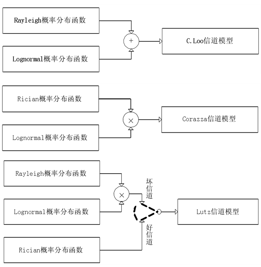
C. Loo模型：直射阴影，多径不阴影
Corazza模型：直射和多径都阴影
Lutz模型：好坏2个状态
Rayleigh and Rician 信道生成
Shadowed-Rician 直射径散射径
- [Secure Transmission in Cognitive Satellite Terrestrial Networks](https://ieeexplore.ieee.org/document/7583691)
- [Resource Allocations for Secure Cognitive Satellite-Terrestrial Networks](https://ieeexplore.ieee.org/document/8048011)
the generalized-K model
Ka频段自由空间损耗雨衰波束增益
L个散射体的阵列响应

比较

C.Loo模型和Corazza模型适用于描述非静止轨道卫星信道的传播特性
Lutz模型适用于描述静止轨道卫星信道的传播特性；
C.Loo模型只适用于乡村信道环境，
而Corazza模型和Lutz模型均适用所有的卫星移动通信信道环境（公路、乡村、郊区和城市）；
C.Loo模型拟合参数时依据的实测数据来自于模拟卫星的直升机所发射的信号；
而Corazza模型和Lutz模型则采用实际卫星所发射信号的实测数据，对卫星移动通信信道传输特性的反映更为真实。

C.Loo	Corazza	Lutz
非静止轨道卫星	非静止轨道卫星	静止轨道卫星
乡村	所有	所有
模拟卫星的直升机	实际卫星	实际卫星

C. Loo模型：直射阴影，多径不阴影

A statistical model for a land mobile satellite link
Chun Loo, “A statistical model for a land mobile satellite link,” in IEEE Transactions on Vehicular Technology, vol. 34, no. 3, pp. 122-127, Aug. 1985, doi: 10.1109/T-VT.1985.24048.

假设接收信号中只有直射信号分量受到阴影遮蔽的作用而多径信号分量不受阴影遮蔽的作用，因此该模型又称为部分阴影信道模型。
C. Loo模型接收信号包络的概率密度函数
${f_r}\left( r \right) = \int_0^\infty {{f_r}\left( {r\left| z \right.} \right){f_z}\left( z \right)dz = \frac{r}{{{{\text{b}}_{\text{0}}}\sqrt {2\pi {d_0}} }}\int_0^\infty {\frac{1}{z}\exp \left[ { - \frac{{{{\left( {\ln z - \mu } \right)}^2}}}{{2{d_0}}} - \frac{{\left( {{r^2} + {z^2}} \right)}}{{2{b_0}}}} \right]} } {\text{dz }}$
z表示直射波，
b0是平均散射多径功率，
μ和d0分别是lnz的均值和方差。

Corazza模型：直射和多径都阴影

假设接收信号中的直射信号分量和多径信号分量同时都受到阴影遮蔽的作用，因此该模型又称为全阴影信道模型
接收信号包络的概率密度函数为
${f_r}\left( r \right) = \int_0^\infty {{f_r}\left( {r\left| s \right.} \right){f_s}\left( s \right)} {\text{ = }}\frac{{{\text{2}}\left( {{\text{k + 1}}} \right)r}}{{h\sigma s\sqrt {2\pi } }}\exp \left( { - k} \right)\int_0^\infty {\exp \left[ { - \frac{{\left( {k + 1} \right){r^2}}}{{{s^2}}} - \frac{{{{\left( {\ln s - \mu } \right)}^2}}}{{2{{\left( {h\sigma } \right)}^2}}}} \right]} {I_0}\left( {\frac{{2r\sqrt {k\left( {k + 1} \right)} }}{s}} \right)ds$
S(t)表示阴影慢衰落效应，
h=(ln10)/20，
μ和σ2为lns的均值和方差，
k为Rice因子，
r为接收信号包络。
${\text{K}}\left( \alpha \right){\text{ = }}{{\text{k}}_{\text{0}}}{\text{ + }}{{\text{k}}_{\text{1}}}\alpha {\text{ + }}{{\text{k}}_{\text{2}}}{\alpha ^{\text{2}}} \\ \mu \left( \alpha \right){\text{ = }}{\mu _{\text{0}}}{\text{ + }}{\mu _{\text{1}}}\alpha {\text{ + }}{\mu _{\text{2}}}{\alpha ^{\text{2}}}{\text{ + }}{\mu _{\text{3}}}{\alpha ^{\text{3}}} \\ \sigma \left( \alpha \right){\text{ = }}{\sigma _{\text{0}}}{\text{ + }}{\sigma _{\text{1}}}\alpha {\text{ }}$

Lutz模型：好坏2个状态

将卫星移动通信信道分为两个状态——“好状态”和“坏状态”。
当信道为“好状态”时接收信号中的直射信号分量和多径信号分量均不受阴影遮蔽的作用；
而当信道为“坏状态”时接收信号中只有受到阴影遮蔽作用的多径信号分量且不存在直射信号分量，因此该模型又称为两状态信道模型。

好状态下接收信号功率S的归一化概率密度函数为
${f_{s\_rician}}\left( s \right) = c\exp \left[ { - c\left( {s + 1} \right)} \right]{I_0}\left( {2c\sqrt s } \right)$
C为归一化因子，c = 1/(2σ2)

坏状态下接收信号功率S的归一化概率密度函数为
${f_{s\_rayl\_LN}}\left( {\text{s}} \right){\text{ = }}\int_{\text{0}}^\infty {{{\text{f}}_{\text{s}}}\left( {s\left| {{s_0}} \right.} \right){f_{s0}}\left( {{s_0}} \right)} {\text{d}}{{\text{s}}_{\text{0}}} \\ {\text{ = }}\frac{{{\text{10}}}}{{\sigma {\text{ln10}}\sqrt {{\text{2}}\pi } }}\int_{\text{0}}^\infty {\frac{{\text{1}}}{{{{\text{s}}_{\text{0}}}^{\text{2}}}}} {\text{exp}}\left[ {{\text{ - }}\frac{{\text{s}}}{{{{\text{s}}_{\text{0}}}}} - \frac{{{{\left( {10{{\log }_{10}}{s_0} - \mu } \right)}^2}}}{{2{\sigma ^2}}}} \right]{\text{ }}$
S0 为短时平均接收功率

总的接收信号功率S的概率密度函数为
$s_rician ( s ) + A f s_rayl_LN ( s ) {f_s}\left( {\text{s}} \right){\text{ = }}\left( {{\text{1 - A}}} \right){{\text{f}}_{{\text{s\_rician}}}}\left( {\text{s}} \right){\text{ + A}}{{\text{f}}_{{\text{s\_rayl\_LN}}}}\left( {\text{s}} \right)$

Rayleigh and Rician 信道生成

2.4.2 Rayleigh and Rician fading
(2.54)
Fundamentals of Wireless Communication

Rayleigh channel (NLoS), Rician channel (LoS)
https://blog.csdn.net/weixin_41181312/article/details/123516627

bandwidth
$B = 180 k Hz$

Noise power spectral density
${N_0} = {10^{\frac{{ - 170}}{{10}}}}mW/Hz$
${N_{0,dBm}} = - 170dBm/Hz$
Noise power
${P_N} = {N_0}B\left( {mW} \right)= {10^{{{ - 170} \over {10}}}} \times 180000\left( {mW} \right)$
${P_{N,dBm}} = 10{\log _{10}}\left( {{P_N}} \right) = {N_{0,dBm}} + 10{\log _{10}}\left( B \right)\left( {dBm} \right) = - 170 + 10{\log _{10}}\left( {180000} \right)\left( {dBm} \right)$

pathloss
$L\left( {d,f} \right) = {\left( {{{4\pi df} \over c}} \right)^2}$
$L_{dB}\left( {d,f} \right) = 10{\log _{10}}\left( {L\left( {d,f} \right)} \right)\left( {dB} \right)$

attenuation
$\alpha \left( {d,f} \right) = \sqrt {L{{\left( {d,f} \right)}^{ - 1}}/P_N} = \sqrt {{{10}^{{{ - L_{dB}\left( {d,f} \right)} \over {10}}}}/{{10}^{{{P_{N,dBm}} \over {10}}}}} = \sqrt {{{10}^{{{ - P_{N,dBm}- L_{dB}\left( {d,f} \right)} \over {10}}}}}$

1 M-antenna transmitter → 1 single-antenna receiver
NLOS
${{\bf{h}}_{NLOS}} = \sqrt {1/2} \left( {{\bf{c}} + j{\bf{e}}} \right) \in {{\Bbb C}^{M \times 1}}$
Rayleigh
${{\bf{h}}_{Rayleigh}}\left( {d,f} \right) = \alpha \left( {d,f} \right){{\bf{h}}_{NLOS}} \in {{\Bbb C}^{M \times 1}}$
Rician
${{\bf{h}}_{Rician}}\left( {d,f} \right) = \alpha \left( {d,f} \right)\left( {\sqrt {\frac{\varepsilon }{{1 + \varepsilon }}} {\bf{a}}\left( \theta \right) + \sqrt {\frac{1}{{1 + \varepsilon }}} {{\bf{h}}_{NLOS}}} \right) \in {{\Bbb C}^{M \times 1}}$

Shadowed-Rician 直射径散射径

优点
计算量小

Although some mathematical models, such as those of Loo, Barts–Stutzman, and Karasawa et al.,have been developed to describe the satellite channel, the shadowed-Rician model proposed in [19] is a popular model, which provides a significantly less computational burden than other channel models.

Secure Transmission in Cognitive Satellite Terrestrial Networks

K. An, M. Lin, J. Ouyang and W. -P. Zhu, “Secure Transmission in Cognitive Satellite Terrestrial Networks,” in IEEE Journal on Selected Areas in Communications, vol. 34, no. 11, pp. 3025-3037, Nov. 2016, doi: 10.1109/JSAC.2016.2615261.

Given a receiver’s position within the satellite spot beam coverage area, the beam gain factor can be approximated as [1], [2]
$b\left ({ \varphi }\right ) = \left ({ {\frac {J_{1}\left ({ u }\right )}{2u} + 36\frac {J_{3}\left ({ u}\right )}{{u_{}^{3}}}} }\right )_{}^{2}$
$2.07123\frac {\sin \varphi }{\sin \varphi _{\mathrm{3dB}}}$
$\varphi$ is the angle between the location of the corresponding receiver and the beam center with respect to the satellite, and $\varphi _{\mathrm{3dB}}$ is the 3-dB angle.

The satellite channels are usually modeled by composite fading distributions to accurately describe the statistical properties of the signal envelope.
Although existing statistical models, such as Loo, Barts-Stutzman, and Karasawa, have been presented to describe the satellite channel, the Shadowed-Rician (SR) model proposed in [33] has been widely used in related work.
In this model, the channel fading coefficient $\bar g$ is described as
$\bar g = A\exp \left ({ {j\psi } }\right ) + Z\exp \left ({ {j\zeta } }\right )$
$ψ$ is a stationary random phase vector with elements uniformly distributed over $[0, 2 π)$ ,
$ζ$ the deterministic phase vector of the LOS component.
$A$ and $Z$ are the amplitudes of the scattering and the LOS components, which are independent stationary random processes following Rayleigh and Nakagami- $m$ distributions respectively.

The SR fading distribution can be characterized as $\bar g} \sim \mathrm {SR}\left ({ {\Omega ,b,m} }\right )$ with
$\Omega$ being the average power of the LoS component,
$2 b$ the average power of the multipath component, and
$m$ the Nakagami- $m$ parameter corresponding to the fading severity.
通过分布函数确定？？

Combining (33) and (35), the overall channel for satellite link can be modeled as
$\sqrt {b\left ({ {\varphi} }\right )} \bar g$

b=0.126
m=10
Omega=0.835
$\varphi _{3\mathrm {dB}}=0.4/180*\pi$

Resource Allocations for Secure Cognitive Satellite-Terrestrial Networks

The SAT is equipped with $N_t$ -antennas
$\mathbf {h}=\sqrt {b(\varphi )}\tilde {\mathbf {h}}$
$b(\varphi )=\left ({\frac {J_{1}(u)}{2u}+36\frac {J_{3}(u)}{u^{3}} }\right )^{2}$
$u=2.07123\frac {\sin \varphi }{\sin \varphi _{3\mathrm {dB}}}$
$\tilde {\mathbf {h}}=A\exp (j\boldsymbol {\psi })\!+\!Z\exp (j\boldsymbol {\phi })$
where $b(\varphi )$ is the corresponding beam gain factor, which is determined by their location.
$\varphi$ is the angle between the corresponding receiver and the beam center, 怎么确定？？
$\varphi _{3\mathrm {dB}}=0.4/180*\pi$ is the 3-dB angle.
$J_{1}(\cdot )$ and $J_{3}(\cdot )$ represent the first-kind Bessel function of order 1 and 3.
$\tilde {\mathbf {h}}\in \mathbb {C}^{N_{t}\times 1}$ denotes the channel fading vector from SAT to the receiver, which include the scattering and the line-of-sight (LOS) components.
$\boldsymbol {\psi }\in [0,2\pi )$ denotes the stationary random phase 随机
$\boldsymbol {\phi }$ denotes the deterministic phase of the LOS component. 怎么确定？？
$A$ and $Z$ are the amplitudes of the scattering and the LOS components. 怎么确定？？
The beam angles from SAT to PU, to Eve and to SU are set as 0.01°, 0.4° and 0.8°, respectively

the generalized-K model

K. P. Peppas, " Accurate closed-form approximations to generalised- $K$ sum distributions and applications in the performance analysis of equal-gain combining receivers ", IET Commun., vol. 5, no. 7, pp. 982-989, May 2011.
I. S. Ansari, S. Al-Ahmadi, F. Yilmaz, M.-S. Alouini, and H. Yanikomeroglu, “A new formula for the BER of binary modulations with dual-branch selection over generalized-K composite fading channels,” IEEE Trans. Commun., vol. 59, no. 10, pp. 2654–2658, Oct. 2011.

Energy Efficient Adaptive Transmissions in Integrated Satellite-Terrestrial Networks With SER Constraints

Y. Ruan, Y. Li, C. -X. Wang, R. Zhang and H. Zhang, “Power Allocation in Cognitive Satellite-Vehicular Networks From Energy-Spectral Efficiency Tradeoff Perspective,” in IEEE Transactions on Cognitive Communications and Networking, vol. 5, no. 2, pp. 318-329, June 2019, doi: 10.1109/TCCN.2019.2905199.

Ka频段自由空间损耗雨衰波束增益

Physical Layer Security in Multibeam Satellite Systems
Ka频段

Z. Lin, M. Lin, J. -B. Wang, T. de Cola and J. Wang, “Joint Beamforming and Power Allocation for Satellite-Terrestrial Integrated Networks With Non-Orthogonal Multiple Access,” in IEEE Journal of Selected Topics in Signal Processing, vol. 13, no. 3, pp. 657-670, June 2019, doi: 10.1109/JSTSP.2019.2899731. 不太一样自由空间损耗雨衰波束增益阵列控制向量
mmWave

M. Lin, C. Yin, Z. Lin, J. -B. Wang, T. de Cola and J. Ouyang, “Combined Beamforming with NOMA for Cognitive Satellite Terrestrial Networks,” ICC 2019 - 2019 IEEE International Conference on Communications (ICC), 2019, pp. 1-6, doi: 10.1109/ICC.2019.8761139.
Ka频段

Joint Beamforming for Secure Communication in Cognitive Satellite Terrestrial Networks
mmWave

the free space loss (FSL)
${C_{L}} = {\left ({{\frac {\lambda }{{4\pi d }}} }\right)^{2}}$

the rain attenuation fading vector ${\mathbf{r}} \in {C^{N_{s} \times 1}}$ between the satellite antenna array and the ground user
${\mathbf{r}} = {\xi ^{ - \frac {1}{2}}}{e^{ - j{\mathbf{p}}}}$
${\mathbf{p}}$ is the ${N_{s}} \times 1$ sized phase vector with its components uniformly distributed over $[0, 2 π)$ 随机
According to ITU-R Recommendation P.1853 [39], the power gain due to rain attenuation in dB, ${\xi _{{\mathrm{dB}}}} = 20{\log _{10}}\left ({\xi }\right)$ , commonly follows a lognormal distribution, namely, ${\mathrm{ln}}\left ({{{\xi _{{\mathrm{dB}}}}} }\right) \sim {\mathcal{ C}}{\mathcal{ N}}\left ({{\mu,{\sigma ^{2}}} }\right)$ , 随机
where $\mu$ and $\sigma$ , both expressed in dB, are the lognormal location and scale parameter, respectively.
$\mu=-3.125$
$\sigma=1.591$

the antenna gain from the $m$ -th on-board beam to the user
${b_{m}} = {b_{\max }}{\left ({{\frac {{J_{1}\left ({{u_{m}} }\right)}}{{2{u_{m}}}} + 36\frac {{J_{3}\left ({{u_{m}} }\right)}}{u_{m}^{3}}} }\right)^{2}}$
${b_{\max }}$ is the maximal satellite antenna gain of the $m$ -th beam,
${u_{m}} = {{2.07123\sin {\phi _{m}}} \mathord {\left /{ {\vphantom {{2.07123\sin {\phi _{m}}} {\sin {{\left ({{{\phi _{{\mathrm{3dB}}}}} }\right)}_{m}}}}} }\right. } {\sin {{\left ({{{\phi _{{\mathrm{3dB}}}}} }\right)}_{m}}}}$ , 怎么确定？？
${J_{1}}\left ({\cdot }\right)$ and ${J_{3}}\left ({\cdot }\right)$ the first-kind Bessel functions of order 1 and 3, respectively.

the overall satellite channel
${\mathbf{f}} = \sqrt {C_{L}} {\mathbf{r}} \odot {{\mathbf{b}}^{\frac {1}{2}}}$
${\mathbf{b}} = {\left [{ {b_{1}, \cdots,{b_{N_{s}}}} }\right]^{T}} \in {C^{N_{s} \times 1}}$ is the beam gain vector

f=20GHz
${b_{\max }}=52dB$
$\varphi _{3\mathrm {dB}}=0.4/180*\pi$
噪声带宽=50MHz

L个散射体的阵列响应

Adaptive scheduling for millimeter wave multi-beam satellite communication systems

Secure Satellite-Terrestrial Transmission Over Incumbent Terrestrial Networks via Cooperative Beamforming
J. Du, C. Jiang, H. Zhang, X. Wang, Y. Ren and M. Debbah, “Secure Satellite-Terrestrial Transmission Over Incumbent Terrestrial Networks via Cooperative Beamforming,” in IEEE Journal on Selected Areas in Communications, vol. 36, no. 7, pp. 1367-1382, July 2018, doi: 10.1109/JSAC.2018.2824623.
mmWave

the channel vector ${{\mathbf {h}}_{n}}\in {{\mathbb {C}}^{{N_{s}}\times 1}}$ of FSS terminal $n$ ( $\in \mathsf {\mathcal {N}} \triangleq \left \{{ 1,2, \cdots,N }\right \}$ )
${{\mathbf {h}}_{n}}=\sqrt {\frac {{N_{s}}}{L}}\sum \nolimits _{l=1}^{L}{{\delta _{n,l}}\boldsymbol {\alpha }\left ({{\theta _{n,l}} }\right)},\quad \forall n\in \mathsf {\mathcal {N}}$
where $L$ is the number of scatters,
${\delta _{n,l}}$ and ${\theta _{n,l}}$ are the complex gain and normalized direction of the LOS path for FSS $n$ , respectively.
In addition, ${\delta _{n,l}^{2}}\sim \mathsf {\mathcal {C}\mathcal {N}}\left ({0,\sigma _{0}^{2} }\right)$ is independent identically distributed (i.i.d.) complex Gaussian distribution with zero-mean, and covariance $\sigma _{0}^{2}=1$ , which indicates Rician factor, and 随机
${\theta _{n,l}}\sim U\left [{ -1,1 }\right]$ is i.i.d. uniformly distributed. 随机
L=2 [36]

Moreover, when a uniform linear array (ULA) is adopted, the normalized array response $α (θ)$ is given by
$\boldsymbol {\alpha }\left ({\theta }\right) = \frac {1}{\sqrt {{N_{s}}}}{{\left [{ 1,{e^{-j\frac {2\pi }{\lambda }d\sin \left ({\varphi }\right)}}, \cdots,{e^{-j\frac {2\pi }{\lambda }\left ({{N_{s}} - 1 }\right)d\sin \left ({\varphi }\right)}} }\right]}^{T}}$
normalized direction $θ n$ is related to the physical azimuth angle of departure (AoD) of $φ \in [- π /2, π /2]$ as $θ = (2 d / λ) s in (φ)$ , 怎么确定？？
where $d$ is the antenna spacing (i.e., the distance between the two adjacent antennas), and
$λ$ is the carrier wavelength.
In this work, we assume the critically sampled environment, i.e, $d / λ = 0.5$ , considering that the normalized AoD is the sine function of the actual AoD.