Week 03 of Advanced Learning Algorithms

笔者在2022年7月份取得这门课的证书，现在（2024年2月25日）才想起来将笔记发布到博客上。

Website: https://www.coursera.org/learn/advanced-learning-algorithms?specialization=machine-learning-introduction

Offered by: DeepLearning.AI and Stanford

课程地址：https://www.coursera.org/learn/machine-learning

本笔记包含字幕，quiz的答案以及作业的代码，仅供个人学习使用，如有侵权，请联系删除。

This week you’ll learn best practices for training and evaluating your learning algorithms to improve performance. This will cover a wide range of useful advice about the machine learning lifecycle, tuning your model, and also improving your training data.

Learning Objectives

---

• Evaluate and then modify your learning algorithm or data to improve your model’s performance
• Evaluate your learning algorithm using cross validation and test datasets.
• Diagnose bias and variance in your learning algorithm
• Use regularization to adjust bias and variance in your learning algorithm
• Identify a baseline level of performance for your learning algorithm
• Understand how bias and variance apply to neural networks
• Learn about the iterative loop of Machine Learning Development that’s used to update and improve a machine learning model
• Learn to use error analysis to identify the types of errors that a learning algorithm is making
• Learn how to add more training data to improve your model, including data augmentation and data synthesis
• Use transfer learning to improve your model’s performance.
• Learn to include fairness and ethics in your machine learning model development
• Measure precision and recall to work with skewed (imbalanced) datasets

[1] Advice for applying machine learning

Deciding what to try next

Debugging a learning algorithm

How do you use learning algorithms effectively?

Hi, and welcome back. By now you’ve seen a lot of different learning algorithms, including linear regression, logistic regression,
even deep learning, or neural networks, and next week, you’ll see
decision trees as well.

You now have a lot of powerful tools of
machine learning, but how do you use these
tools effectively?

Depend to a large part on how well you can repeatedly make good decisions

I’ve seen teams sometimes, say six months to build a
machine learning system, that I think a more
skilled team could have taken or done in just
a couple of weeks.

The efficiency of
how quickly you can get a machine learning
system to work well, will depend to a large part on how well you can
repeatedly make good decisions about
what to do next in the course of a
machine learning project.

In this week, I hope to share with you a
number of tips on how to make decisions
about what to do next in machine
learning project, that I hope will end up
saving you a lot of time.

Let’s take a look at some advice on how to build
machine learning systems.

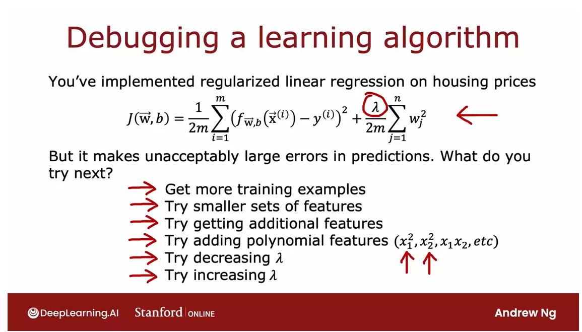
Let’s start with an example, say you’ve implemented
regularized linear regression to predict housing prices, so you have the
usual cost function for your learning algorithm, squared error plus this
regularization term.

Example: unacceptably large errors in prediction

But if you train the model, and find that it makes unacceptably large errors
in it’s predictions, what do you try next?

When you’re building a
machine learning algorithm, there are usually a lot of different things
you could try.

For example, you
could decide to get more training examples since it seems having more
data should help, or maybe you think maybe
you have too many features, so you could try a
smaller set of features.

Or maybe you want to get
additional features, such as finally
additional properties of the houses to
toss into your data, and maybe that’ll help
you to do better.

Or you might take the
existing features x_1, x_2, and so on, and try adding polynomial
features x_1 squared, x_2 squared, x_1,
x_2, and so on.

Or you might wonder if the value of Lambda is chosen well, and you might say, maybe it’s too big, I want
to decrease it. Or you may say, maybe
it’s too small, I want to try increasing.

On any given machine
learning application, it will often turn
out that some of these things could be fruitful, and some of these
things not fruitful.

Find a way to make good choices

The key to being effective
at how you build a machine learning algorithm
will be if you can find a way to make good choices about where
to invest your time.

For example, I have
seen teams spend literally many months collecting
more training examples, thinking that more training
data is going to help, but it turns out
sometimes it helps a lot, and sometimes it doesn’t.

Machine learning diagnostic

In this week, you’ll
learn about how to carry out a set of diagnostic.

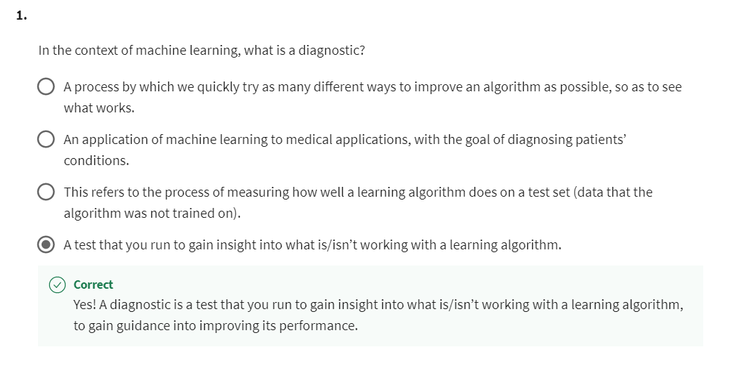
Diagnostic： a test that you can run to gain insight into what is or isn’t working with learning algorithm to gain guidance into improving its performance.

By diagnostic, I mean
a test that you can run to gain insight into what is or isn’t working
with learning algorithm to gain guidance into improving its performance.

Some of these diagnostics
will tell you things like, is it worth weeks,
or even months collecting more training
data, because if it is, then you can then
go ahead and make the investment to get more data, which will hopefully lead
to improved performance, or if it isn’t then running that diagnostic could have
saved you months of time.

One thing you see
this week as well, is that diagnostics can
take time to implement, but running them can be a
very good use of your time.

This week we’ll spend
a lot of time talking about different
diagnostics you can use, to give you guidance on how to improve your learning
algorithm’s performance. But first, let’s take
a look at how to evaluate the performance of
your learning algorithm. Let’s go do that
in the next video.

Evaluating a model

Let’s see,
you’ve trained a machine learning model. How do you evaluate that
model’s performance?

You find that having a systematic way to
evaluate performance will also hope paint a clearer path for
how to improve his performance. So let’s take a look at
how to evaluate the model.

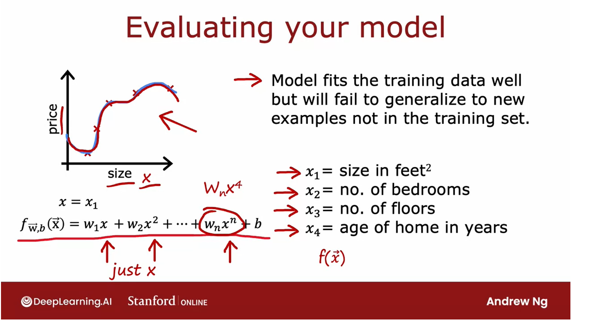
Let’s take the example of learning
to predict housing prices as a function of the size. Let’s say you’ve trained the model
to predict housing prices as a function of the size x. And for the model that is
a fourth order polynomial.

So features x, x squared,
execute and x to the 4. Because we fit 1/4 order polynomial to
a training set with five data points, this fits the training data really well.

But, we don’t like this model
very much because even though the model fits the training data well, we think it will fail to generalize to new
examples that aren’t in the training set.

So, when you are predicting prices, just
a single feature at the size of the house, you could plot the model like this and we
could see that the curve is very weakly so we know this parody isn’t a good model.

But if you were fitting this
model with even more features, say we had x1 the size of house,
number of bedrooms, the number of floors of the house,
also the age of the home in years, then it becomes much harder to plot f because
f is now a function of x1 through x4.

And how do you plot a four
dimensional function?

So in order to tell if your model is doing
well, especially for applications where you have more than one or two features,
which makes it difficult to plot f of x.

We need some more systematic way to
evaluate how well your model is doing.

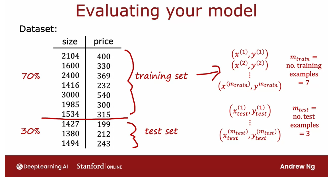
Here’s a technique that you can use. If you have a training set and this is
a small training set with just 10 examples listed here, rather than taking all
your data to train the parameters w and p of the model, you can instead split
the training set into two subsets.

I’m going to draw a line here, and
let’s put 70% of the data into the first part and
I’m going to call that the training set.

And the second part of the data,
let’s say 30% of the data, I’m going to put into it has set.

And what we’re going to
do is train the models, parameters on the training set on
this first 70% or so of the data, and then we’ll test his
performance on this test set.

In notation, I’m going to use x1, why 1? Same as before, to denote
the training examples through xm, ym, except that now to make explicit.

So in this little example we would
have seven training example.

And to introduce one
new piece of notation, I’m going to use m subscript train. M train is a number of training examples
which in this small dataset is 7. So the subscript train just
emphasizes if we’re looking at the training set portion of the data.

And for the test set, I’m going to use
the notation x1 subscript test comma y1, subscript test to denote
the first test example, and this goes all the way to
x m test subscript tests. Why m test?

Subscript tests and m tests is the number
of test examples, which in this case is 3.

And it’s not uncommon to split your
dataset according to maybe a 70, 30 split or 80, 20 split with most of
your data going into the training set, and then a smaller fraction
going into the test set.

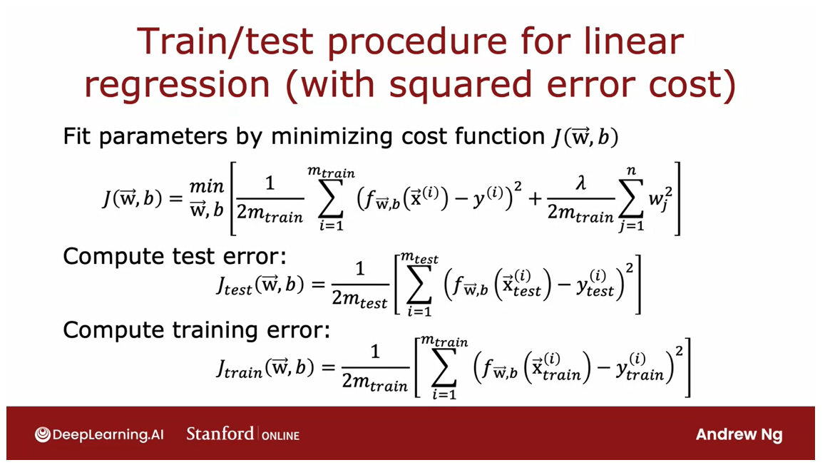
So, in order to train a model and
evaluated it, this is what it would look like if you’re using linear
regression with a squared error cost.

Start off by fitting the parameters by
minimizing the cost function j of w,b. So this is the usual cost
function minimize over w,b of this square error cost,
plus regularization term longer over 2m times
some of the w,j squared.

And then to tell how well this model is
doing, you would compute J test of w,b, which is equal to the average
error on the test set, and that’s just equal to 1/2 times m test. That’s the number of test examples.

And then of some overall the examples
from r equals 1, to the number of test examples of the squared era
on each of the test examples like so.

So it’s a prediction on the if
test example input minus the actual price of the house
on the test example squared. And notice that the test
error formula J test, it does not include that
regularization term.

And this will give you a sense of how
well your learning algorithm is doing.

One of the quantity that’s often
useful to computer as well as the training error,
which is a measure of how well you’re learning algorithm is doing
on the training set.

So let me define J train of w,b
to be equal to the average over the training set. 1 over to 2m, or 1/2 m subscript train of some over your training set
of this squared error term.

And once again, this does not include
the regularization term unlike the cost function that you are minimizing
to fit the parameters.

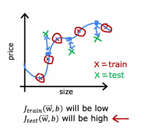
So, in the model like what we
saw earlier in this video, J train of w,b will be low
because the average era on your training examples will be zero or
very close to zero.

So J train will be very close to zero. But if you have a few additional examples
in your test set that the algorithm had not trained on, then those test examples,
my love life these.

And there’s a large gap between what
the algorithm is predicting as the estimated housing price, and
the actual value of those housing prices.

And so, J tests will be high. So seeing that J test is high on this
model, gives you a way to realize that even though it does great on the training
set, is actually not so good at generalizing to new examples to new data
points that were not in the training set.

So, that was regression
with squared error cost.

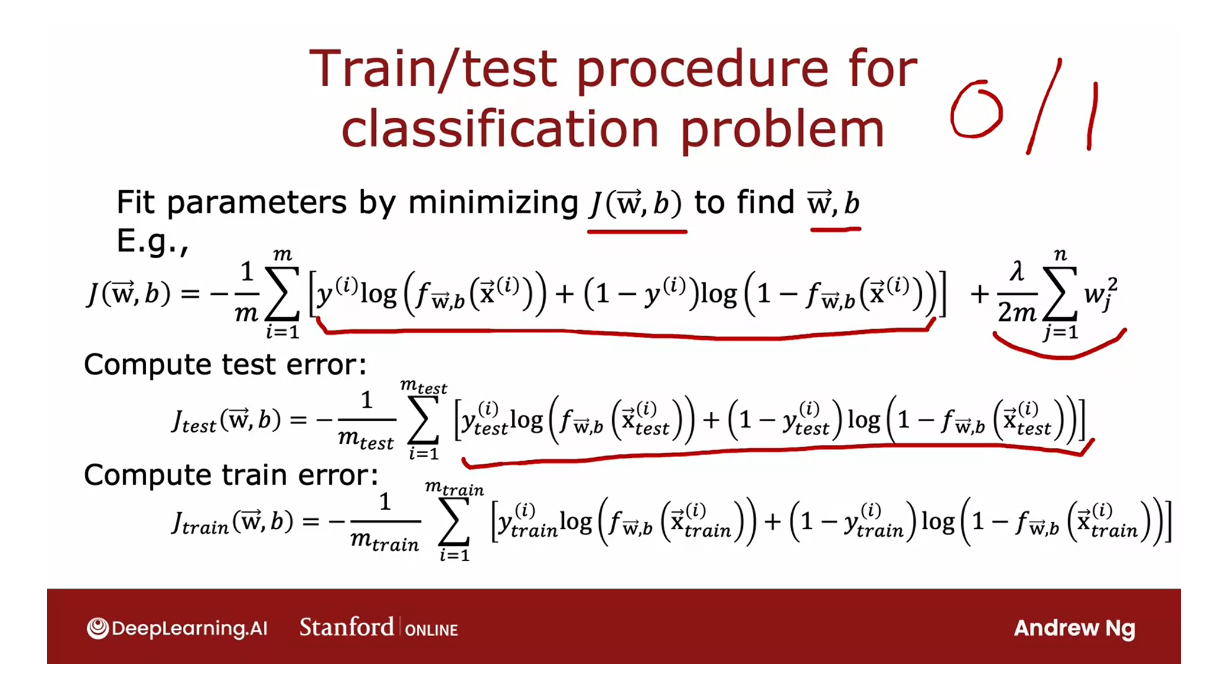
Procedure of classification problem

Now, let’s take a look at how you apply
this procedure to a classification problem.

For example, if you are classifying
between handwritten digits that are either 0 or
1, so same as before, you fit the parameters by minimizing the
cost function to find the parameters w,b.

For example,
if you were training logistic regression, then this would be the cost function
J of w,b, where this is the usual logistic loss function, and
then plus also the regularization term.

And to compute the test error,
J test is then the average over your test examples,
that’s that 30% of your data that wasn’t in the training set of the logistic
loss on your test set.

And the training error you can
also compute using this formula, is the average logistic loss
on your training data that the algorithm was using to minimize
the cost function J of w, b.

Well, when I described here will work,
okay, for figuring out if your learning algorithm is doing well, by seeing how
I was doing in terms of test error.

When applying machine learning
to classification problems, there’s actually one other
definition of J tests and J train that is maybe
even more commonly used.

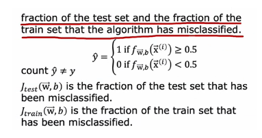
Which is instead of using the logistic
loss to compute the test error and the training error to instead measure
what the fraction of the test set, and the fraction of the training set
that the algorithm has misclassified.

So specifically on the chess set,
you can have the algorithm make a prediction 1 or
0 on every test example.

So, recall why hat we would predict us
1 if f of x is greater than equal 4.5, and zero if it’s less than 0.5.

And you can then count up in the test
set the fraction of examples where why hat is not equal to the actual
ground truth label while in the test set.

So concretely, if you are classifying
handwritten digits 0, 1 by new classification toss, then J tests
would be the fraction of that test set, where 0 was classified as 1 of 1,
classified as 0. And similarly, J train is a fraction of the training
set that has been misclassified.

Taking a dataset and splitting it into a
training set and a separate test set gives you a way to systematically evaluate
how well your learning outcomes doing.

By computing both J tests and J train, you can now measure how was doing on
the test set and on the training set.

This procedure is one step to what you’ll
be able to automatically choose what model to use for
a given machine learning application.

For example, if you’re trying
to predict housing prices, should you fit a straight
line to your data, or fit a second order polynomial, or
third order fourth order polynomial?

It turns out that with one further
refinement to the idea you saw in this video, you’ll be able to have an algorithm
help you to automatically make that type of decision well. Let’s take a look at how to
do that in the next video.

Model selection and training/cross validation/test sets

Automatically choose a good model for the machine learning algorithm

In the last video,
you saw how to use the test set to evaluate
the performance of a model.

Let’s make one
further refinement to that idea in this video, which allow you to
use the technique, to automatically
choose a good model for your machine
learning algorithm.

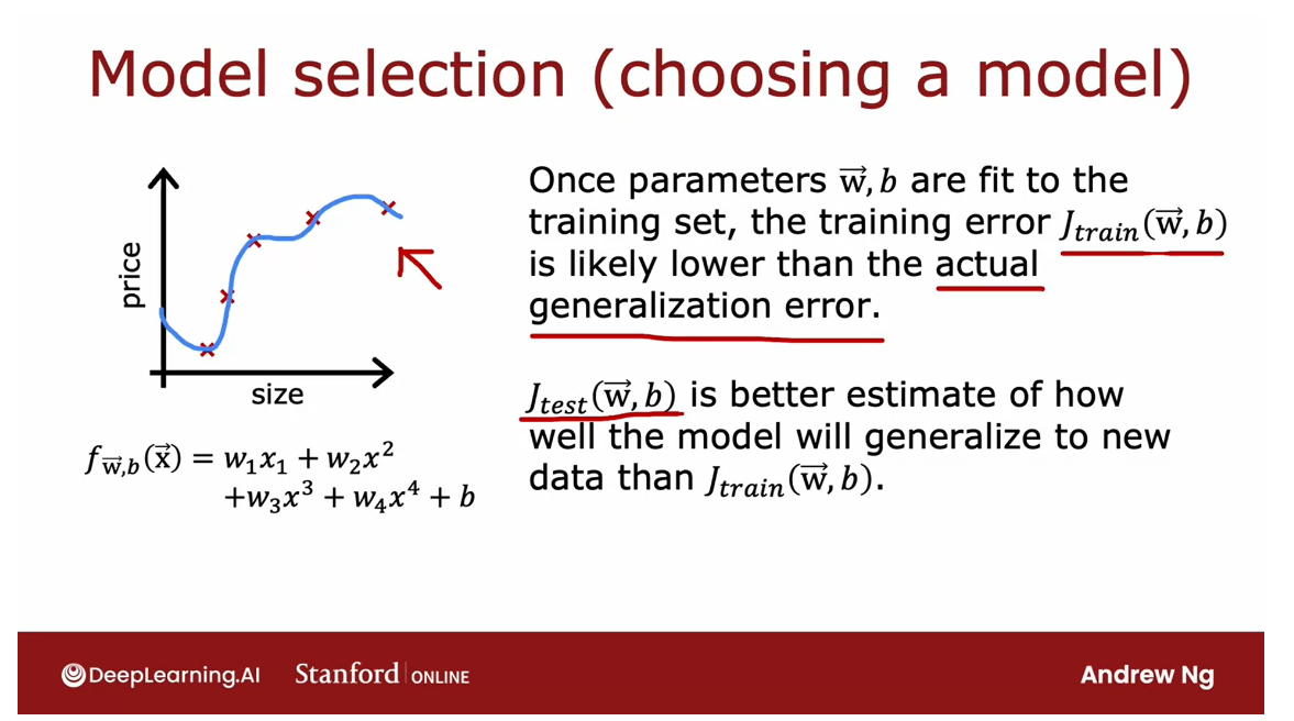
One thing we’ve
seen is that once the model’s parameters w and b have been fit to
the training set.

The training error may not be a good indicator of how
well the algorithm will do or how well it
will generalize to new examples that were
not in the training set, and in particular,
for this example, the training error will
be pretty much zero.

That’s likely much lower than the actual generalization error, and by that I mean
the average error on new examples that were
not in the training set.

What you saw on the
last video is that J test the performance of
the algorithm on examples, is not trained on, that will be a
better indicator of how well the model will
likely do on new data.

Let’s take a look at how to use a test set to choose a model for a given machine learning application

By that I mean other data
that’s not in the training set. Let’s take a look at
how this affects, how we might use a test set to choose a model for a given
machine learning application.

If a fitting a function to predict housing prices or some
other regression problem, one model you might consider is to fit a linear
model like this.

This is a first-order
polynomial and we’re going to use d equals 1 on this slide to denote fitting a one or
first-order polynomial.

If you were to fit a model like this to
your training set, you get some
parameters, w and b, and you can then compute J tests to estimate how well does this
generalize to new data?

On this slide, I’m
going to use w^1, b^1 to denote that these
are the parameters you get if you were to fit a
first order polynomial, a degree one, d
equals 1 polynomial.

Now, you might also consider fitting a second-order
polynomial or quadratic model, so this is the model. If you were to fit this
to your training set, you would get some
parameters, w^2, b^2, and you can then
similarly evaluate those parameters on your
test set and get J test w^2, b^2, and this will give
you a sense of how well the second-order
polynomial does.

You can go on to try d equals 3, that’s a third order or a degree three polynomial
that looks like this, and fit parameters and
similarly get J test.

You might keep doing this until, say you try up to a 10th
order polynomial and you end up with J test
of w^10, b^10.

That gives you a
sense of how well the 10th order
polynomial is doing.

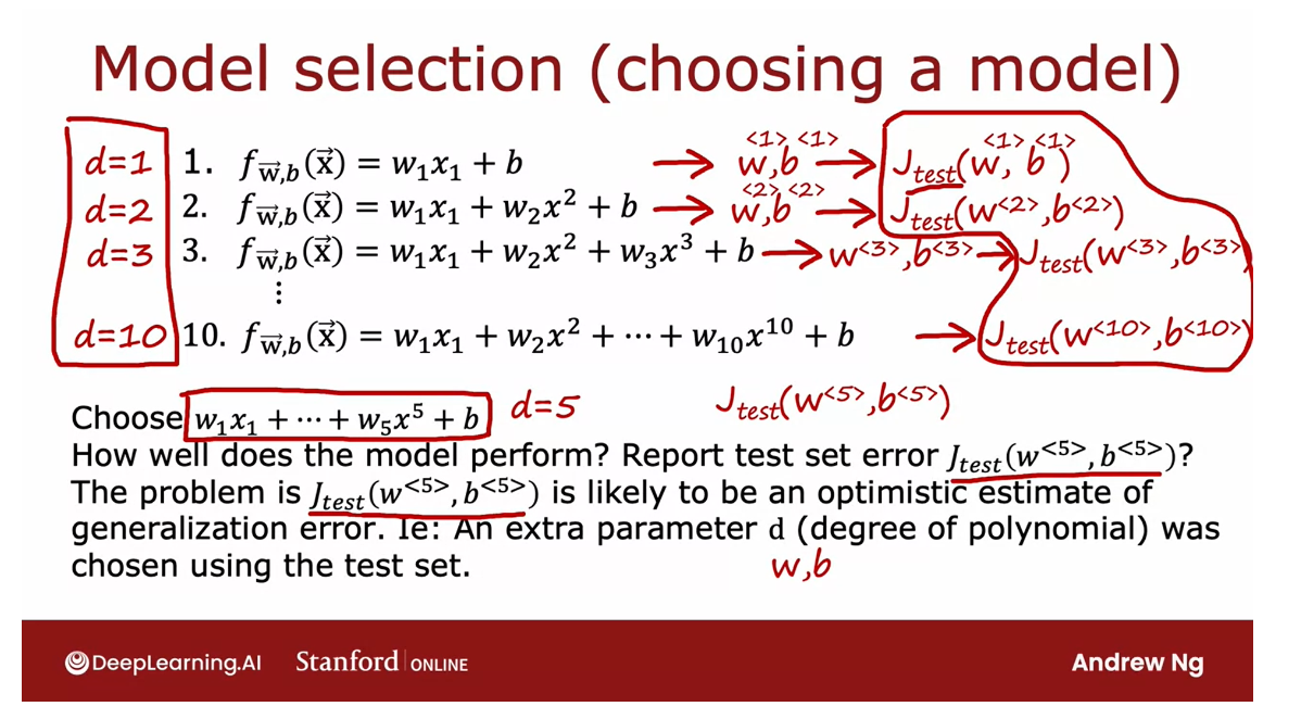
One procedure you could try, this turns out not to
be the best procedure, but one thing you could try is, look at all of these J tests, and see which one gives
you the lowest value.

If $J_{test}$ is the lowest => it does best

Say, you find that, J test for the fifth
order polynomial for w^5, b^5 turns out to be the lowest. If that’s the case, then
you might decide that the fifth order polynomial
d equals 5 does best, and choose that model
for your application.

To report the test test error

If you want to estimate how
well this model performs, one thing you could do, but this turns out to be a
slightly flawed procedure, is to report the test set error, J test w^5, b^5.

The reason this procedure
is flawed is J test of w^5, b^5 is likely to be an optimistic estimate of
the generalization error.

$J_{test}$ is likely to be an optimistic estimate of the generalization error

In other words, it
is likely to be lower than the actual
generalization error, and the reason is, in the procedure we talked
about on this slide with basic fits, one
extra parameter, which is d, the
degree of polynomial, and we chose this parameter
using the test set.

On the previous slide, we saw
that if you were to fit w, b to the training data, then the training data would be an overly optimistic estimate
of generalization error.

It turns out too, that if
you want to choose the parameter d using the test set, then the test set J test is
now an overly optimistic, that is lower than
actual estimate of the generalization error.

Cross validation

validation set = development set = dev set

The procedure on this
particular slide is flawed and I don’t
recommend using this.

Instead, if you want to
automatically choose a model, such as decide what
degree polynomial to use.

Here’s how you modify
the training and testing procedure in order to
carry out model selection.

Whereby model selection, I mean choosing amongst
different models, such as these 10 different
models that you might contemplate using for your
machine learning application.

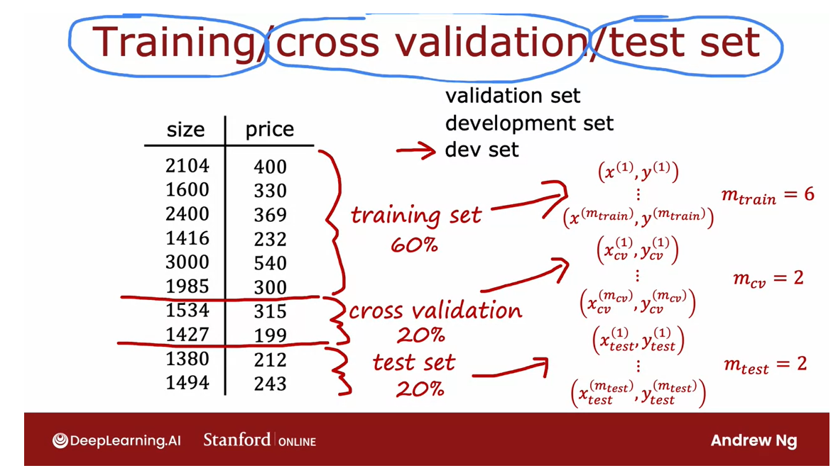
Splitting our data into three different subsets

The way we’ll modify the
procedure is instead of splitting your data
into just two subsets, the training set
and the test set, we’re going to split your data into three different subsets, which we’re going to
call the training set, the cross-validation set,
and then also the test set.

Using our example from before of these 10 training examples, we might split it into putting 60 percent
of the data into the training set and so the notation we’ll use for the training set portion
will be the same as before, except that now M train, the number of training
examples will be six and we might put 20
percent of the data into the cross-validation set and a notation I’m going
to use is x_cv of one, y_cv of one for the first
cross-validation example.

So cv stands for
cross-validation, all the way down to x_cv
of m_cv and y_cv of m_cv.

Where here, m_cv equals
2 in this example, is the number of
cross-validation examples.

Then finally we have the
test set same as before, so x1 through x m tests
and y1 through y m, where m tests equal to 2. This is the number
of test examples.

We’ll see you on the
next slide how to use the cross-validation set.

The way we’ll modify
the procedure is you’ve already seen
the training set and the test set and we’re
going to introduce a new subset of the data called
the cross-validation set.

Cross-validation: an extra dataset used to check the validity or the accuracy of different models

The name cross-validation
refers to that this is an extra dataset
that we’re going to use to check or trust check the validity or really the
accuracy of different models.

I don t think it’s a great name, but that is what people
in machine learning have gotten to call
this extra dataset.

You may also hear people call this the validation
set for short, it’s just fewer syllables than cross-validation or
in some applications, people also call this
the development set.

Means basically the same
thing or for short.

Sometimes you hear people
call this the dev set, but all of these terms mean the same thing as
cross-validation set.

I personally use the term dev set the most often because
it’s the shortest, fastest way to say it but
cross-validation is pretty used a little bit more often by machine learning
practitioners.

Onto these three subsets
of the data training set, cross-validation
set, and test set, you can then compute the training error, the
cross-validation error, and the test error using
these three formulas.

None of these three terms include the regularization term

The regularization term is only included in the training objective.

Whereas usual, none of
these terms include the regularization term that is included in the
training objective, and this new term in the middle, the cross-validation error
is just the average over your m_cv
cross-validation examples of the average say,
squared error.

This term, in addition to being called
cross-validation error, is also commonly called the
validation error for short, or even the development set
error, or the dev error.

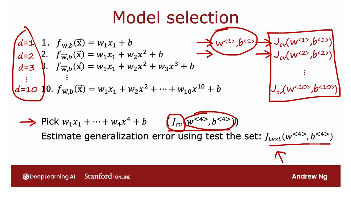
Armed with these three measures of learning algorithm
performance, this is how you can then go about carrying out
model selection.

You can, with the 10 models, same as earlier on this slide, with d equals 1, d equals 2, all the way up to a 10th degree or the
10th order polynomial, you can then fit the
parameters w_1, b_1.

But instead of evaluating
this on your test set, you will instead evaluate
these parameters on your cross-validation sets
and compute J_cv of w1, b1, and similarly, for the second model, we get J_cv of w2, v2, and all the way down
to J_cv of w10, b10.

Then, in order to
choose a model, you will look at which model has the lowest
cross-validation error, and concretely, let’s
say that J_cv of w4, b4 as low as, then what that means is you pick this fourth-order polynomial as the model you will use
for this application.

Finally, if you want to
report out an estimate of the generalization error of how well this model will
do on new data.

You will do so using that
third subset of your data, the test set and you
report out Jtest of w4,b4. You notice that throughout
this entire procedure, you had fit these parameters
using the training set.

You then chose the parameter
d or chose the degree of polynomial using the
cross-validation set and so up until this point, you’ve not fit any parameters, either w or b or d to the test set and that’s why
Jtest in this example will be fair estimate of the generalization error of this model thus
parameters w4,b4.

This gives a better procedure for model selection
and it lets you automatically make a
decision like what order polynomial to choose for your
linear regression model.

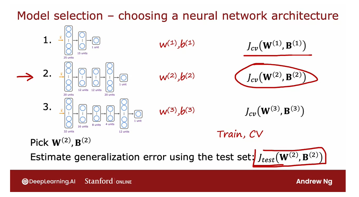
This model selection
procedure also works for choosing among
other types of models.

For example, choosing a
neural network architecture.

If you are fitting a model for handwritten
digit recognition, you might consider
three models like this, maybe even a larger set of
models than just me but here are a few different
neural networks of small, somewhat larger, and
then even larger.

To help you decide
how many layers do the neural network have and how many hidden units per
layer should you have, you can then train all
three of these models and end up with parameters w1, b1 for the first model, w2, b2 for the second model, and w3,b3 for the third model.

You can then evaluate the neural networks
performance using Jcv, using your cross-validation set and where the
classification problem, Jcv can be the
percentage of examples.

Since this is a
classification problem, Jcv the most common choice
would be to compute this as the fraction of
cross-validation examples that the algorithm
has misclassified.

Pick a model? with the lowest cross validation error

Report out an estimate of the generalization error: use the test set to estimate

You would compute this using all three models and then pick the model with the lowest
cross validation error.

If in this example, this has the lowest
cross validation error, you will then pick the second
neural network and use parameters trained on
this model and finally, if you want to report out an estimate of the
generalization error, you then use the test set to estimate how well
the neural network that you just chose will do.

Make decisions only looking at the training set and cross-validation set

After all the decisions, evaluate them on the test set.

In machine learning practice
is considered best practice to make all the decisions you want to make regarding
your learning algorithm, such as how to
choose parameters, what degree polynomial to use, but make decisions
only looking at the training set and
cross-validation set and to not use the test set at all
to make decisions about your model and only after you’ve made
all those decisions,

then finally, tick
them all though you have designed and evaluated
on your test set.

That procedure ensures
that you haven’t accidentally fit anything
to the test set so that your test set becomes so unfair and not overly
optimistic estimate of generalization error
of your algorithm.

It’s considered best
practice in machine learning that if you have to make
decisions about your model, such as fitting parameters or choosing the model architecture, such as neural network
architecture or degree of polynomial if you’re fitting
a linear regression, to make all those
decisions only using your training set and your
cross-validation set, and to not look at the test
set at all while you’re still making decisions regarding
your learning algorithm.

It’s only after
you’ve come up with one model as your final
model to only then evaluate it on the test set and because you haven’t made any decisions using the test set, that ensures that
your test set is a fair and not overly
optimistic estimate of how well your model will
generalize to new data.

That’s model
selection and this is actually a very widely
used procedure. I use this all the
time to automatically choose what model to use for a given machine
learning application.

Earlier this week, I mentioned
running diagnostics to decide how to improve the performance of a
learning algorithm.

Now that you have
a way to evaluate learning algorithms and even automatically choose a model, let’s dive more deeply into
examples of some diagnostics.

The most powerful diagnostic that I know of and that
I used for a lot of machine learning
applications is one called bias and variance. Let’s take a look at what
that means in the next video.

[2] Practice quiz: Advice for applying machine learning

Practice quiz: Advice for applying machine learning

Latest Submission Grade 100%

Actually, if a model overfits the training set, it may not generalize well to new data.

Question 3

For a classification task; suppose you train three different models using three different neural network architectures. Which data do you use to evaluate the three models in order to choose the best one?

Incorrect. You’ll only use the test set after choosing the best model based on the cross validation set. You want to avoid using the test set while you are still selecting model options, because the test set is meant to serve as an estimate for how the model will generalize to new examples that it has never seen before.

Correct. Use the cross validation set to calculate the cross validation error on all three models in order to compare which of the three models is best.

[3] Bias and variance

Diagnosing bias and variance

The typical workflow
of developing a machine learning
system is that you have an idea and
you train the model, and you almost
always find that it doesn’t work as well
as you wish yet.

When I’m training a
machine learning model, it pretty much never works
that well the first time.

Bias and variance of a learning algorithm gives you very good guidance on what to try next

Key to the process of building machine learning
system is how to decide what to do next in order to improve
his performance.

I’ve found across many
different applications that looking at the bias and variance of a learning
algorithm gives you very good guidance
on what to try next.

Let’s take a look
at what this means.

You might remember
this example from the first course on
linear regression.

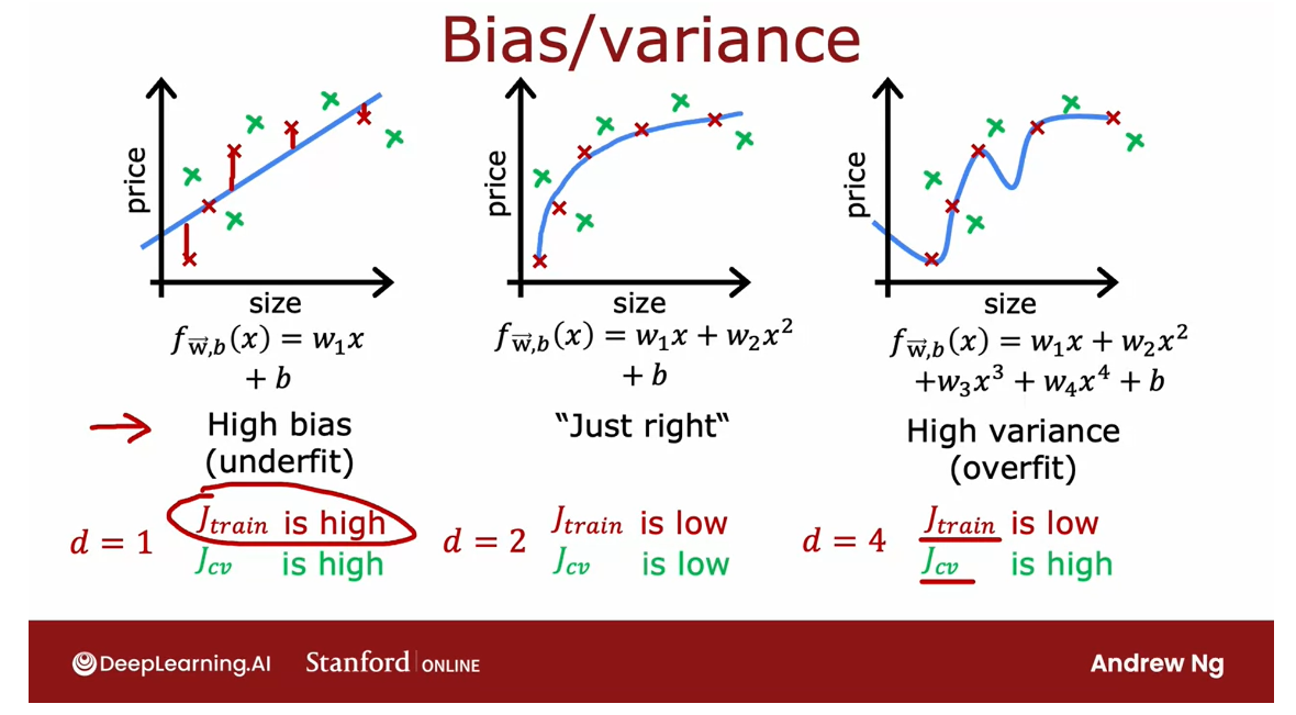
Where given this dataset, if you were to fit a
straight line to it, it doesn’t do that well. We said that this algorithm has high bias or that it
underfits this dataset.

If you were to fit a
fourth-order polynomial, then it has high-variance
or it overfits.

In the middle if you fit
a quadratic polynomial, then it looks pretty good. Then I said that was just right. Because this is a problem
with just a single feature x, we could plot the function
f and look at it like this.

If more features, we can’t plot and visualize whether it’s doing well as easily.

Diagnose: look at bias and variance on the training set and on the cross validation set

But if you had more features, you can’t plot f and visualize whether it’s
doing well as easily.

Instead of trying to
look at plots like this, a more systematic way to diagnose or to find out if your algorithm
has high bias or high variance will be to
look at the performance of your algorithm on
the training set and on the cross validation set.

In particular, let’s look
at the example on the left.

If you were to compute J_train, how well does the algorithm
do on the training set? Not that well.

I’d say J train here would be high
because there are actually pretty large errors between the examples and the actual
predictions of the model.

How about J_cv? J_cv would be if we had
a few new examples, maybe examples like that, that the algorithm had
not previously seen.

Here the algorithm
also doesn’t do that well on examples that it
had not previously seen, so J_cv will also be high.

Underfit: high bias

It’s not even doing well on the training set

One characteristic of an
algorithm with high bias, something that is under fitting, is that it’s not even doing that well on
the training set.

When J_train is high, that is your strong indicator that this algorithm
has high bias.

Let’s now look at the
example on the right. If you were to compute J_train, how well is this doing
on the training set?

Well, it’s actually doing
great on the training set. Fits the training
data really well. J_train here will be low.

But if you were to evaluate this model on other houses
not in the training set, then you find that J_cv, the cross-validation
error, will be quite high.

Overfit: high variance

It does much better on data it has seen than on data it has not seen.

A characteristic signature or a characteristic Q that
your algorithm has high variance will be of J_cv is much higher
than J_train.

In other words, it does
much better on data it has seen than on data
it has not seen.

This turns out to be a strong indicator that your
algorithm has high variance.

Again, the point of
what we’re doing is that I’m computing J_train and J_cv and seeing if J _train is high or if J_cv is
much higher than J_train.

This gives you a sense, even if you can’t
plot to function f, of whether your algorithm has
high bias or high variance.

Just right: doesn’t have a high bias problem or high variance problem.

Finally, the chase
in the middle. If you look at J_train, it’s pretty low,
so this is doing quite well on the training set.

If you were to look at
a few new examples, like those from, say, your cross-validation set, you find that J_cv is
also a pretty low.

J_train not being too high indicates this doesn’t have
a high bias problem and J_cv not being much worse than J_train this indicates that it doesn’t have a high
variance problem either.

Which is why the quadratic model seems to be a pretty good
one for this application.

Let me share with you another
view of bias and variance.

To summarize, when d equals
1 for a linear polynomial, J_train was high
and J_cv was high. When d equals 4, J train was low, but J_cv is high.

When d equals 2, both were pretty low. Let’s now take a different
view on bias and variance. In particular, on
the next slide I’d like to show you how J_train and J_cv variance as a function of the degree of the
polynomial you’re fitting.

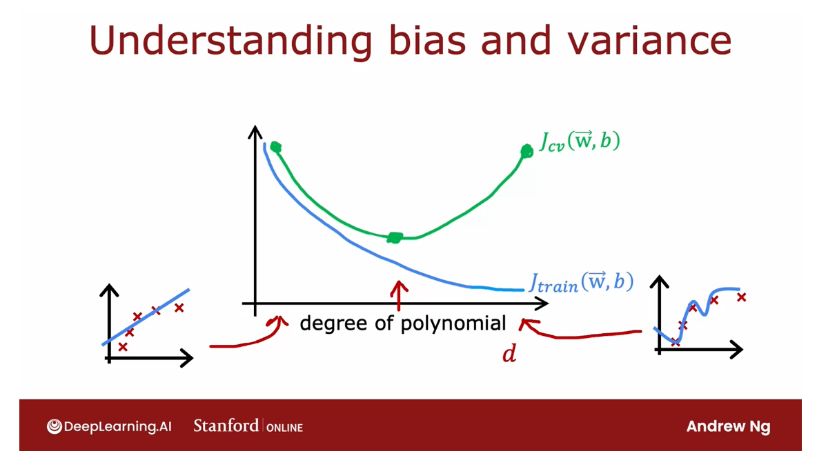
Plot a function of the degree of polynomial

Let me draw a figure where the horizontal
axis, this d here, will be the degree of polynomial that we’re fitting to the data.

Over on the left we’ll correspond
to a small value of d, like d equals 1, which corresponds to
fitting straight line.

Over to the right we’ll
correspond to, say, d equals 4 or even
higher values of d. We’re fitting this
high order polynomial.

So if you were to
plot J train or W, B as a function of the
degree of polynomial, what you find is that as you fit a higher and higher
degree polynomial, here I’m assuming we’re
not using regularization, but as you fit a higher and
higher order polynomial, the training error
will tend to go down because when you have a very
simple linear function, it doesn’t fit the
training data that well, when you fit a
quadratic function or third order polynomial or
fourth-order polynomial, it fits the training
data better and better.

As the degree of
polynomial increases, J train will typically go down.

Next, let’s look at J_cv, which is how well does it do on data that it did
not get to fit to?

What we saw was
when d equals one, when the degree of
polynomial was very low, J_cv was pretty high
because it underfits, so it didn’t do well on
the cross validation set.

Here on the right as well, when the degree of polynomial
is very large, say four, it doesn’t do well on the
cross-validation set either, and so it’s also high.

Vary the degree of polynomial, get a curve

But if d was in-between say, a second-order polynomial, then it actually
did much better. If you were to vary the
degree of polynomial, you’d actually get a curve
that looks like this, which comes down and
then goes back up.

Where if the degree of
polynomial is too low, it underfits and so doesn’t
do the cross validation set, if it is too high, it overfits and also doesn’t do well on the cross
validation set.

Is only if it’s
somewhere in the middle, that is just right, which is why the
second-order polynomial in our example ends up with a lower cross-validation
error and neither high bias
nor high-variance.

How to diagnose bias and variance in the learning algorithm?

To summarize, how
do you diagnose bias and variance in
your learning algorithm?

If your learning algorithm has high bias or it has
undefeated data, the key indicator will
be if J train is high.

That corresponds to this
leftmost portion of the curve, which is where J train as high.

Usually you have J train and J_cv will be close
to each other.

How do you diagnose if
you have high variance?

While the key indicator
for high-variance will be if J_cv is much greater than J train does double greater than sign in math
refers to a much greater than, so this is greater, and this means much greater.

This rightmost portion
of the plot is where J_cv is much greater
than J train.

Usually J train
will be pretty low, but the key indicator is whether J_cv is much greater
than J train. That’s what happens when we had fit a very high order polynomial
to this small dataset.

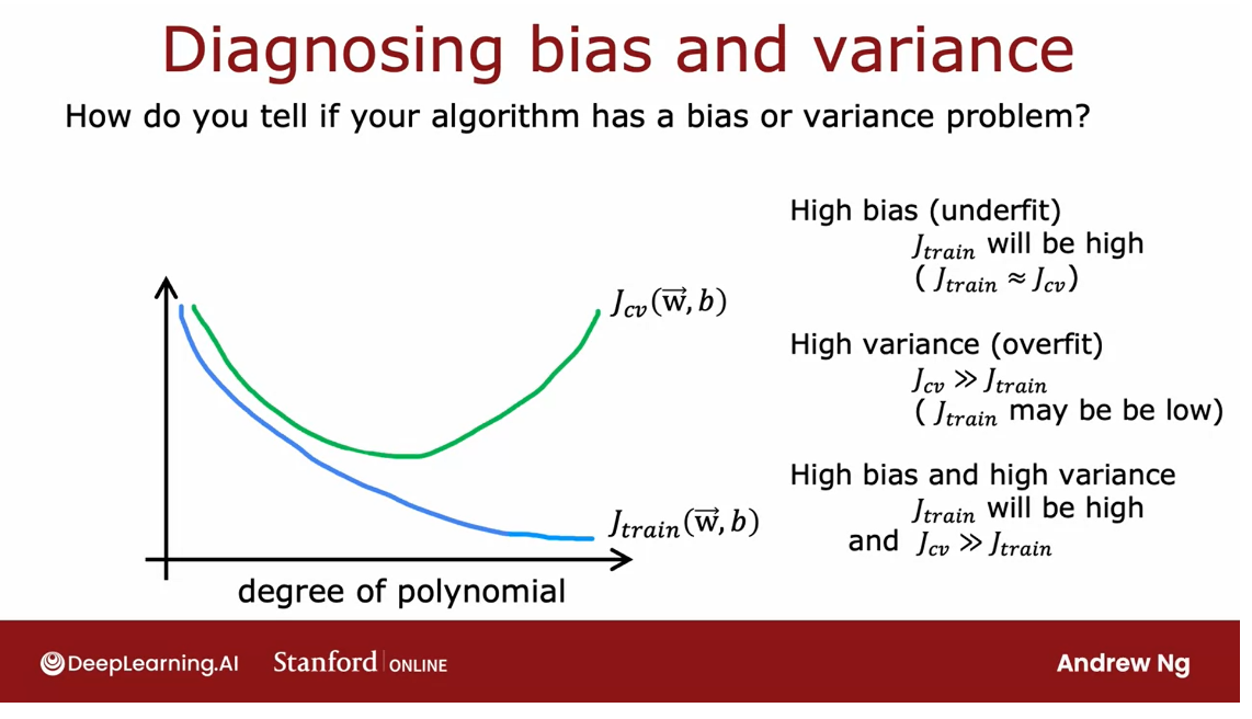
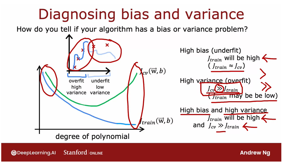
High bias and high variance

Even though we’ve just
seen bias in the areas, it turns out, in some cases, is possible to simultaneously have high bias and
have high-variance.

You won’t see this happen that much for linear regression, but it turns out that if you’re training
a neural network, there are some
applications where unfortunately you have high
bias and high variance.

One way to recognize
that situation will be if J train is high, so you’re not doing that well on the training set,
but even worse, the cross-validation
error is again, even much larger than
the training set.

The notion of high bias
and high variance, it doesn’t really happen for linear models
applied to one deep.

Intuition about both high bias and high variance.

But to give intuition
about what it looks like, it would be as if for
part of the input, you had a very complicated
model that overfit, so it overfits to
part of the inputs.

But then for some reason, for other parts of the input, it doesn’t even fit the
training data well, and so it underfits
for part of the input.

In this example, which
looks artificial because it’s a single
feature input, we fit the training
set really well and we overfit in
part of the input, and we don’t even fit
the training data well, and we underfit the
part of the input.

That’s how in some
applications you can unfortunate end up with both
high bias and high variance.

The indicator for
that will be if the algorithm does poorly
on the training set, and it even does much worse
than on the training set.

For most learning applications, you probably have
primarily a high bias or high variance problem rather than both
at the same time.

But it is possible sometimes they’re both
at the same time.

The key takeaways

I know that there’s
a lot of process, there are a lot of
concepts on the slides, but the key takeaways are, high bias means is not even doing well on
the training set, and high variance means, it does much worse on the cross validation set
and the training set.

Whenever I’m training a
machine learning algorithm, I will almost always
try to figure out to what extent
the algorithm has a high bias or underfitting versus a high-variance
when overfitting problem.

This will give good guidance, as we’ll see later this week, on how you can improve the
performance of the algorithm.

But first, let’s take a look at how regularization
effects the bias and variance of a learning algorithm
because that will help you better understand when you
should use regularization. Let’s take a look at
that in the next video.

Regularization and bias/variance

You saw in the last video how different choices
of the degree of polynomial D affects the bias and variance of your
learning algorithm and therefore its
overall performance.

In this video, let’s take a
look at how regularization, specifically the choice of the regularization
parameter Lambda affects the bias
and variance and therefore the overall
performance of the algorithm.

This, it turns out, will be helpful
for when you want to choose a good value of Lambda of the
regularization parameter for your algorithm.
Let’s take a look.

In this example, I’m going to use a fourth-order polynomial, but we’re going to fit this
model using regularization.

Where here the value of Lambda is the regularization
parameter that controls how much you trade-off
keeping the parameters w small versus fitting
the training data well.

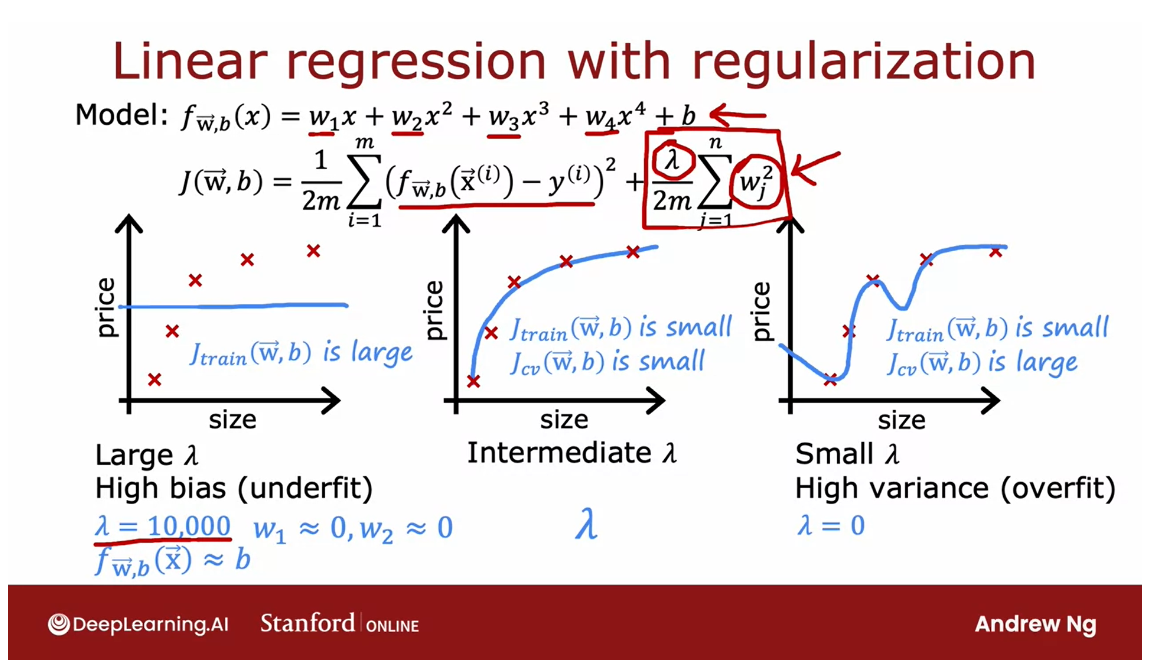
Let’s start with the
example of setting Lambda to be a very large value.

Say Lambda is equal to 10,000. If you were to do so, you would end up fitting a model that looks
roughly like this.

Because if Lambda
were very large, then the algorithm is
highly motivated to keep these parameters w very small and so you
end up with w_1, w_2, really all of these parameters will
be very close to zero.

The model ends up
being f of x is just approximately
b a constant value, which is why you end up
with a model like this.

This model clearly has
high bias and it underfits the training data because
it doesn’t even do well on the training set and
J_train is large.

Let’s take a look at
the other extreme. Let’s say you set Lambda
to be a very small value.

With a small value of Lambda, in fact, let’s go to extreme of setting Lambda equals zero.

With that choice of Lambda, there is no regularization, so we’re just fitting a
fourth-order polynomial with no regularization
and you end up with that curve that you saw previously that
overfits the data.

What we saw previously was when you have
a model like this, J_train is small, but J_cv is much larger than
J_train or J_cv is large.

This indicates we
have high variance and it overfits this data.

It would be if you have some intermediate
value of Lambda, not really largely 10,000, but not so small as zero that hopefully you get a model
that looks like this, that is just right and
fits the data well with small J_train
and small J_cv.

If you are trying
to decide what is a good value of Lambda to use for the
regularization parameter, cross-validation gives you
a way to do so as well.

Using regularization, how can you choose a good value of lambda?

Let’s take a look at
how we could do so.

Just as a reminder, the problem we’re addressing is if you’re fitting a
fourth-order polynomial, so that’s the model and
you’re using regularization, how can you choose a
good value of Lambda?

This would be procedures similar
to what you had seen for choosing the degree of polynomial D using
cross-validation.

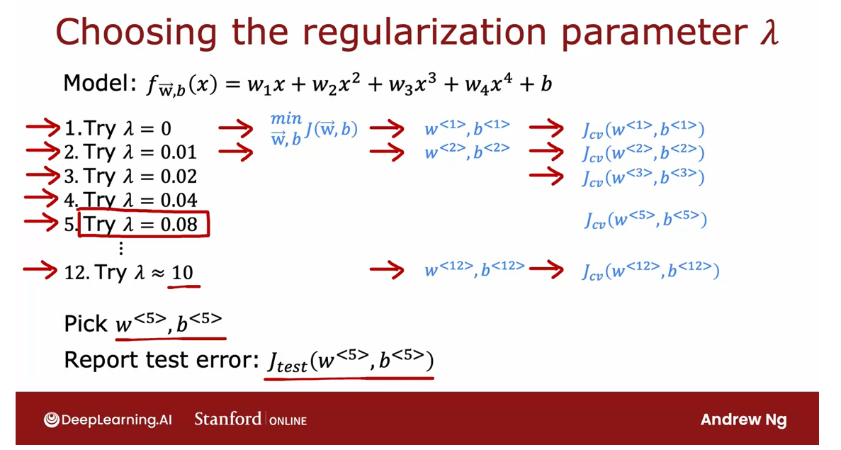
Specifically, let’s
say we try to fit a model using
Lambda equals 0.

We would minimize
the cost function using Lambda equals 0 and end
up with some parameters w1, b1 and you can then compute
the cross-validation error, J_cv of w1, b1.

Now let’s try a different
value of Lambda. Let’s say you try
Lambda equals 0.01.

Then again, minimizing
the cost function gives you a second set
of parameters, w2, b2 and you can also see how well that does on the
cross-validation set, and so on.

Let’s keep trying
other values of Lambda and in this example, I’m going to try doubling
it to Lambda equals 0.02 and so that will
give you J_cv of w3, b3, and so on. Then let’s double again
and double again.

After doubling a
number of times, you end up with Lambda
approximately equal to 10, and that will give
you parameters w12, b12, and J_cv w12 of b12.

By trying out a large range of possible values for Lambda, fitting parameters using those different
regularization parameters, and then evaluating
the performance on the cross-validation set, you can then try to pick what is the best value for the
regularization parameter.

Quickly. If in this example, you find that J_cv of W5, B5 has the lowest value of all of these different
cross-validation errors, you might then decide to
pick this value for Lambda, and so use W5, B5 as to chosen parameters.

Finally, if you want to report out an estimate of the
generalization error, you would then report
out the test set error, J tests of W5, B5.

How training error and cross validation error vary as a function of the parameter lambda

To further hone intuition about what this
algorithm is doing, let’s take a look at how training error and
cross validation error vary as a function of
the parameter Lambda.

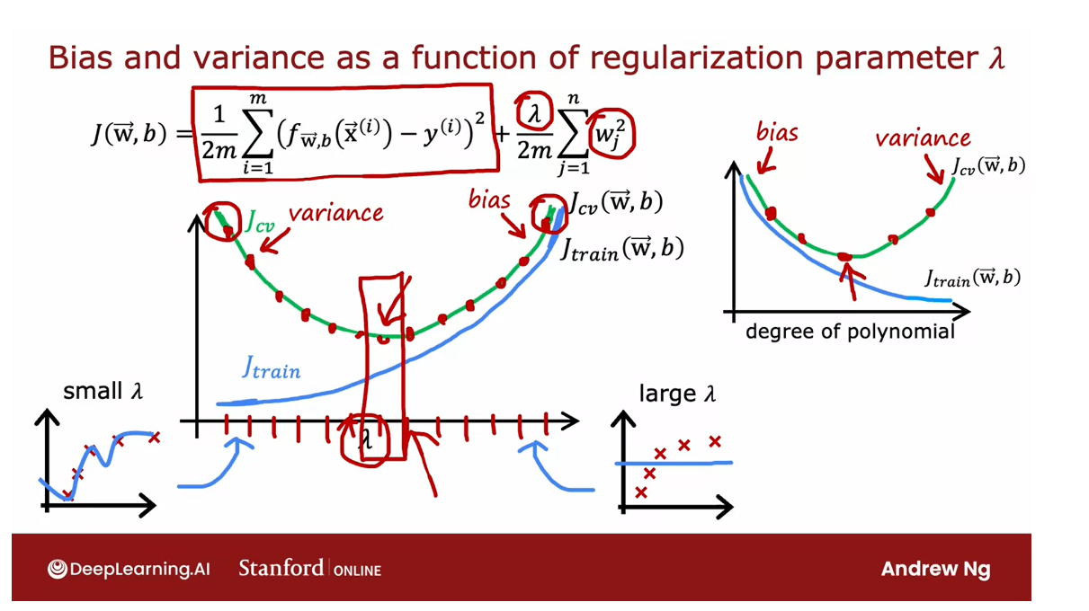
In this figure, I’ve
changed the x-axis again.

Notice that the x-axis here is annotated with the value of the regularization
parameter Lambda, and if we look at the extreme of Lambda equals zero
here on the left, that corresponds to not
using any regularization, and so that’s where we wound up with this very wiggly curve.

If Lambda was small
or it was even zero, and in that case, we have a high variance model, and so J train is going to be small and J_cv is going to be large because it does great on the training data but does much worse on the cross
validation data.

Large lambda: High bias, underfit the data

as Lambda increases, the training error J train will tend to increase

This extreme on the right were very large
values of Lambda. Say Lambda equals 10,000 ends up with fitting a model
that looks like that.

This has high bias, it underfits the data, and it turns out J
train will be high and J_cv will be high as well.

In fact, if you
were to look at how J train varies as a
function of Lambda, you find that J train
will go up like this because in the
optimization cost function, the larger Lambda is, the more the algorithm is
trying to keep W squared small.

That is, the more weight is given to this
regularization term, and thus the less
attention is paid to actually do well
on the training set.

This term on the
left is J train, so the most trying to keep
the parameters small, the less good a job it does on minimizing
the training error.

That’s why as Lambda increases, the training error J train
will tend to increase like so.

Now, how about the
cross-validation error?

Turns out the cross-validation
error will look like this. Because we’ve seen that if Lambda is too small
or too large, then it doesn’t do well on
the cross-validation set.

It either overfits here on the left or underfits
here on the right.

There’ll be some intermediate
value of Lambda that causes the algorithm
to perform best.

What cross-validation
is doing is, it’s trying out a lot of
different values of Lambda.

This is what we saw
on the last slide; trial Lambda equals zero, Lambda equals 0.01,
logic is 0,02.

Try different values of lambda and evaluate the cross validation errors

Try a lot of different
values of Lambda and evaluate the
cross-validation error in a lot of these
different points, and then hopefully pick a value that has low cross
validation error, and this will hopefully correspond to a good model
for your application.

If you compare this diagram to the one that we had in
the previous video, where the horizontal axis was
the degree of polynomial, these two diagrams look a little bit not mathematically and
not in any formal way, but they look a little bit like mirror images
of each other, and that’s because when you’re fitting a
degree of polynomial, the left part of this
curve corresponded to overfitting in high bias, the right part corresponded to underfitting in high variance.

Whereas in this one, high-variance was
on the left and high bias was on the right.

But that’s why these two
images are a little bit like mirror images
of each other.

You can use cross-validation to make a good choice for the regularization parameter Lambda.

But in both cases,
cross-validation, evaluating different
values can help you choose a good value of degree
or a good value of Lambda.

That’s how the choice of regularization parameter
Lambda affects the bias and variance and overall performance
of your algorithm, and you’ve also seen how you
can use cross-validation to make a good choice for the regularization
parameter Lambda.

Now, so far, we’ve talked about how having
a high training set error, high J train is indicative of high bias and how having a high cross-validation
error of J_cv, specifically if it’s much
higher than J train, how that’s indicative
of variance problem.

But what does these
words “high” or “much higher” actually mean?

Let’s take a look at that in the next video where we’ll
look at how you can look at the numbers J train and J_cv and judge if
it’s high or low, and it turns out that one further refinement
of these ideas, that is, establishing a baseline level of performance we’re learning algorithm will make it much easier for you to look
at these numbers, J train, J_cv, and judge if they
are high or low. Let’s take a look at what all this means in the next video.

Establishing a baseline level of performance

Let’s look at some
concrete numbers for what J-train and JCV might be, and see how you can judge if a learning algorithm has
high bias or high variance.

Example: application of speech recognition

For the examples in this video, I’m going to use as a running
example the application of speech recognition which is something I’ve worked on
multiple times over the years. Let’s take a look.

A lot of users doing web search on a
mobile phone will use speech recognition
rather than type on the tiny keyboards on
our phones because speaking to a phone is
often faster than typing.

Typical audio that’s
a web search engine we get would be like this, “What is today’s weather?” Or like this, “Coffee shops near me.” It’s the job of the speech recognition algorithms to output the transcripts whether it’s today’s weather or
coffee shops near me.

Now, if you were to train a speech recognition system and measure the training error, and the training
error means what’s the percentage of audio clips in your training set that
the algorithm does not transcribe correctly
in its entirety.

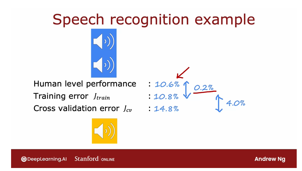
Let’s say the training error for this data-set is
10.8 percent meaning that it transcribes it perfectly for 89.2 percent of
your training set, but makes some mistake in 10.8 percent of
your training set.

If you were to also measure your speech recognition
algorithm’s performance on a separate
cross-validation set, let’s say it gets
14.8 percent error.

If you were to look at these numbers it looks like the training error
is really high, it got 10 percent wrong, and then the cross-validation
error is higher but getting 10 percent of even
your training set wrong that seems pretty high.

It seems like that 10 percent
error would lead you to conclude it has high bias because it’s not doing
well on your training set, but it turns out
that when analyzing speech recognition
it’s useful to also measure one other
thing which is what is the human level of performance?

what is the human level of performance

In other words, how
well can even humans transcribe speech accurately
from these audio clips?

Concretely, let’s
say that you measure how well fluent speakers can transcribe audio
clips and you find that it is 10.6 percent, and you find that human
level performance achieves 10.6 percent error.

Why is human level
error so high? It turns out that
for web search, there are a lot of audio
clips that sound like this, “I’m going to navigate
to [inaudible].”

There’s a lot of
noisy audio where really no one can accurately transcribe what was said because of the
noise in the audio.

If even a human makes
10.6 percent error, then it seems difficult to expect a learning algorithm
to do much better.

In order to judge if the
training error is high, it turns out to be
more useful to see if the training error is much higher than a human
level of performance, and in this example it does just 0.2 percent
worse than humans.

Given that humans are
actually really good at recognizing speech I think if I can build a speech recognition
system that achieves 10.6 percent error matching human performance
I’d be pretty happy, so it’s just doing a little
bit worse than humans.

But in contrast, the
gap or the difference between JCV and J-train
is much larger. There’s actually a four
percent gap there, whereas previously
we had said maybe 10.8 percent error means
this is high bias.

When we benchmark it to
human level performance, we see that the
algorithm is actually doing quite well on
the training set, but the bigger problem is the cross-validation
error is much higher than the
training error which is why I would conclude that this algorithm actually has more of a variance problem
than a bias problem.

by baseline level of performance I mean what is the level of error you can reasonably hope your learning algorithm to eventually get to.

It turns out when judging if the training error is high is often useful to establish a baseline level of performance, and by baseline level
of performance I mean what is the level of error you can
reasonably hope your learning algorithm to
eventually get to.

One common way to establish a baseline level of performance
is to measure how well humans can do on
this task because humans are really good at
understanding speech data, or processing images or
understanding texts.

Human level performance is often a good benchmark when you
are using unstructured data, such as: audio, images, or texts.

Another way to estimate a baseline level
of performance is if there’s some
competing algorithm, maybe a previous implementation that someone else has
implemented or even a competitor’s
algorithm to establish a baseline level of performance
if you can measure that, or sometimes you might guess
based on prior experience.

If you have access to this baseline level of
performance that is, what is the level of error you can reasonably
hope to get to or what is the desired level of performance that you want
your algorithm to get to?

Then when judging if an algorithm has high
bias or variance, you would look at the baseline
level of performance, and the training error, and the cross-validation error.

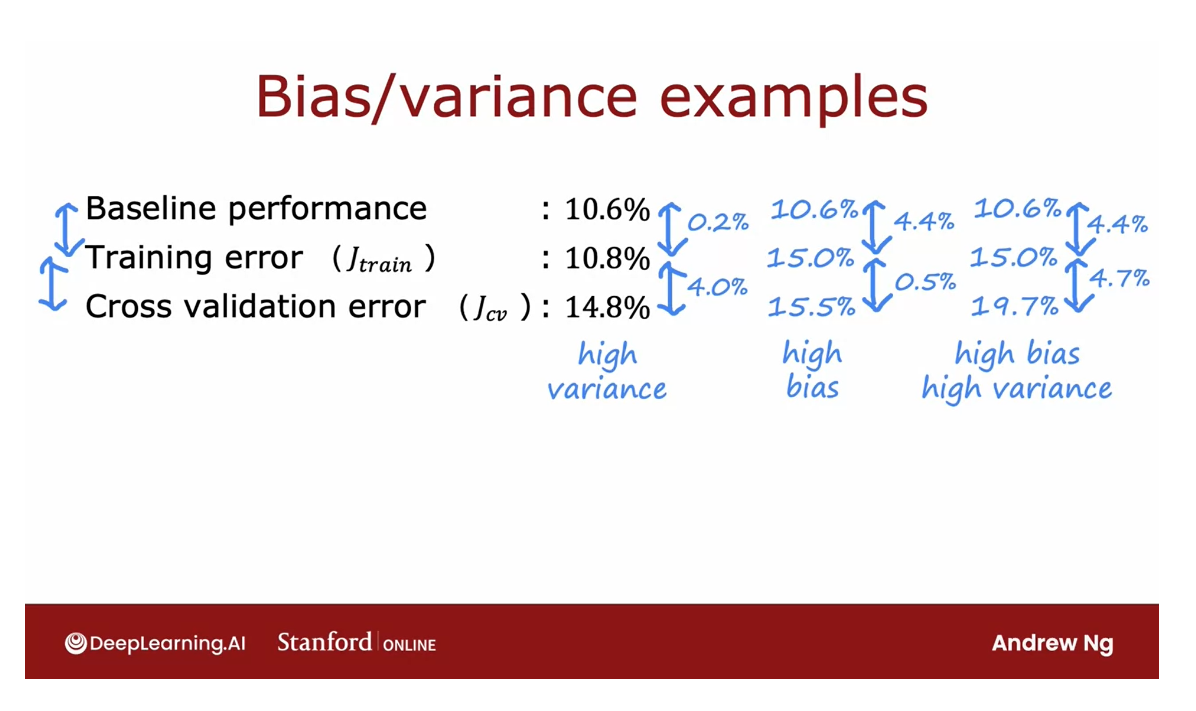
The two key quantities
to measure are then: what is the difference between training error and the baseline level that
you hope to get to.

This is 0.2, and if this is large then you would say you have
a high bias problem. You will then also look at this gap between
your training error and your cross-validation error, and if this is high then you will conclude you have a
high variance problem.

That’s why in this example we concluded we have a
high variance problem, whereas let’s look at
the second example. If the baseline level
of performance; that is human level performance,
and training error, and cross validation
error look like this, then this first gap is 4.4 percent and so
there’s actually a big gap.

The training error
is much higher than what humans can
do and what we hope to get to whereas the
cross-validation error is just a little bit bigger
than the training error.

If your training error and cross validation
error look like this, I will say this
algorithm has high bias.

By looking at these numbers, training error and
cross validation error, you can get a sense
intuitively or informally of the degree to which
your algorithm has a high bias or
high variance problem.

Just to summarize,
this gap between these first two
numbers gives you a sense of whether you
have a high bias problem, and the gap between these
two numbers gives you a sense of whether you have
a high variance problem.

Sometimes the baseline level of performance could
be zero percent.

If your goal is to achieve perfect performance
than the baseline level of performance it
could be zero percent, but for some applications like the speech recognition
application where some audio is just noisy then
the baseline level of a performance could be
much higher than zero.

The method described
on this slide will give you a better read in terms of whether your algorithm suffers from bias or variance.

By the way, it is possible for your algorithms to have high
bias and high variance.

Concretely, if you get
numbers like these, then the gap between the baseline and the
training error is large. That would be a 4.6 percent, and the gap between training error and cross
validation error is also large. This is 4.2 percent.

If it looks like this
you will conclude that your algorithm has high
bias and high variance, although hopefully
this won’t happen that often for your
learning applications.

To summarize, we’ve seen that looking at whether
your training error is large is a way to tell if
your algorithm has high bias, but on applications
where the data is sometimes just noisy
and is infeasible or unrealistic to
ever expect to get a zero error then it’s useful to establish this baseline
level of performance.

Rather than just asking is
my training error a lot, you can ask is my training error large relative to what I hope
I can get to eventually, such as, is my training large relative to what
humans can do on the task?

That gives you a more
accurate read on how far away you are in terms of your training error from
where you hope to get to.

Then similarly, looking at whether your
cross-validation error is much larger than
your training error, gives you a sense
of whether or not your algorithm may have a high
variance problem as well.

In practice, this is how I often will look at these
numbers to judge if my learning algorithm has a high bias or high
variance problem.

Now, to further hone our intuition about how a
learning algorithm is doing, there’s one other
thing that I found useful to think about which
is the learning curve. Let’s take a look at what
that means in the next video.

Learning curves

Learning curve: function of the amount of experience (for example, the number of training examples)

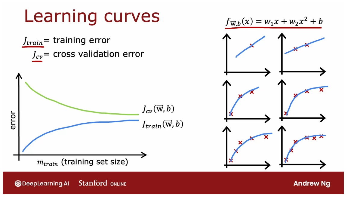
Learning curves are a way
to help understand how your learning
algorithm is doing as a function of the amount
of experience it has, whereby experience, I mean, for example, the number of
training examples it has.

Let’s take a look. Let me
plot the learning curves for a model that fits a second-order polynomial
quadratic function like so.

I’m going to plot both J_cv, the cross-validation error, as well as J_train
the training error. On this figure, the
horizontal axis is going to be m_train.

That is the training set size or the number of examples so the
algorithm can learn from.

On the vertical axis, I’m going to plot the error. By error, I mean either
J_cv or J_train.

Let’s start by plotting the
cross-validation error. It will look
something like this. That’s what J_cv of
(w, b) will look like.

Is maybe no surprise
that as m_train, the training set
size gets bigger, then you learn a better model and so the cross-validation
error goes down.

Now, let’s plot J_train of (w, b) of what the training
error looks like as the training set
size gets bigger.

It turns out that
the training error will actually look like this. That has the training
set size gets bigger, the training set error
actually increases.

Let’s take a look at
why this is the case. We’ll start with an example of when you have just a
single training example.

Well, if you were to fit a
quadratic model to this, you can fit easiest
straight line or a curve and your training
error will be zero.

How about if you have two
training examples like this? Well, you can again fit a straight line and achieve
zero training error.

In fact, if you have
three training examples, the quadratic function
can still fit this very well and get pretty much
zero training error, but now, if your training set
gets a little bit bigger, say you have four
training examples, then it gets a
little bit harder to fit all four examples perfectly.

You may get a curve
that looks like this, is a pretty well, but you’re a little bit off in a few
places here and there.

When you have entries, the training set size to four the training error has
actually gone up a little bit.

How about we have five
training examples. Well again, you can
fit it pretty well, but it gets even a
little bit harder to fit all of them perfectly.

We haven’t even larger shading sets it just gets harder and harder to fit every single one of your training
examples perfectly.

To recap, when you have
a very small number of training examples like
one or two or even three, is relatively easy to get zero or very
small training error, but when you have a
larger training set is harder for quadratic function to fit all the training
examples perfectly.

Which is why as the
training set gets bigger, the training error
increases because it’s harder to fit all of the
training examples perfectly.

Notice one other thing
about these curves, which is the
cross-validation error, will be typically higher than the training error because you fit the parameters
to the training set.

You expect to do
at least a little bit better or when m is small, maybe even a lot better on the training set than on
the trans validation set.

High Bias 欠拟合 underfit

Let’s now take a look at what the learning curves
will look like for an average with high bias versus
one with high variance.

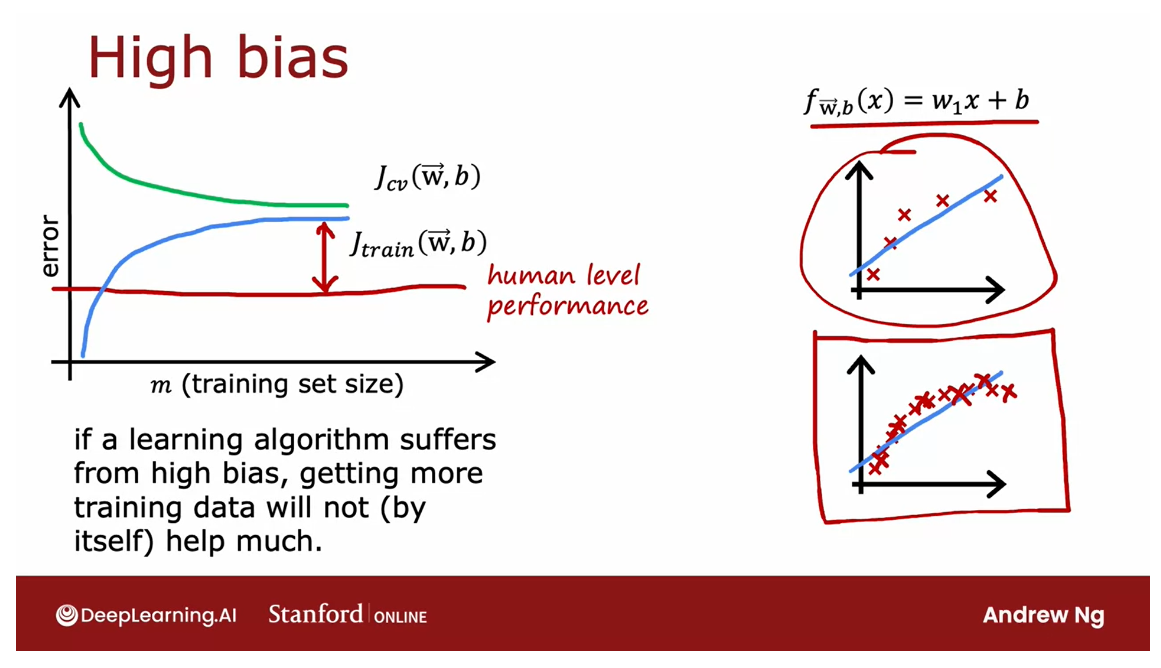
Let’s start at the high bias
or the underfitting case.

Recall that an example of high bias would be if you’re
fitting a linear function, so curve that looks like this. If you were to plot
the training error, then the training error will go up like so as you’d expect.

In fact, this curve of training error may
start to flatten out. We call it plateau, meaning flatten
out after a while.

That’s because as you get more and more training examples when you’re fitting the
simple linear function, your model doesn’t actually
change that much more.

Average training error flattens out after a while

Cross validation error come down and also flattened out after a while

It’s fitting a straight
line and even as you get more and more
and more examples, there’s just not that
much more to change, which is why the
average training error flattens out after a while.

Similarly, your cross-validation
error will come down and also flattened
out after a while, which is why J_cv again
is higher than J_train, but J_cv will tend
to look like that.

It’s because be
honest, its endpoints, even as you get more and
more and more examples, not much is going to change about the street
now you’re fitting.

It’s just too simple a model to be fitting into
this much data. Which is why both of
these curves, J_cv, and J_train tend to
flatten after a while.

Have a measure of the baseline level of performance

Big gap between the baseline level of performance and $J_{train}$: indicator for this algorithm having high bias

If you had a measure of that baseline
level of performance, such as human-level performance, then they’ll tend to
be a value that is lower than your
J_train and your J_cv.

Human-level performance
may look like this.

There’s a big gap between the baseline level of
performance and J_train, which was our indicator for this algorithm having high bias. That is, one could hope to
be doing much better if only we could fit a more complex function
than just a straight line.

Now, one interesting thing about this plot is you can ask, what do you think
will happen if you could have a much
bigger training set?

What would it look
like if we could increase even further than
the right of this plot, you can go further to
the right as follows?

Well, you can imagine if you were to extend both of
these curves to the right, they’ll both flatten out
and both of them will probably just continue
to be flat like that.

No matter how far you
extend to the right of this plot, these two curves, they will never somehow
find a way to dip down to this human level
performance or just keep on being flat like this, pretty much forever no matter how large the training set gets.

That gives this conclusion, maybe a little bit surprising, that if a learning
algorithm has high bias, getting more training
data will not by itself hope that much.

High bias: more data will not let you bring down the error rate that much

I know that we’re
used to thinking that having more data is good, but if your algorithm
has high bias, then if the only thing you do is throw more
training data added, that by itself will not ever let you bring down the
error rate that much.

It’s because of this really, no matter how many more examples
you add to this figure, the straight linear
fitting just isn’t going to get that much better.

That’s why before
investing a lot of effort into collecting
more training data, it’s worth checking if your learning algorithm has high bias, because if it does, then you probably need to do some other things other than just throw more
training data added.

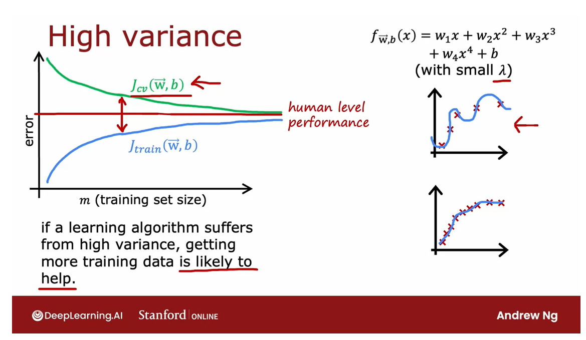
High Variance

Overfit 过拟合的情况

Let’s now take a look at what the learning curve
looks like for learning algorithm
with high variance.

You might remember that
if you were to fit the forefather polynomial
with small lambda, say, or even lambda equals zero, then you get a curve
that looks like this, and even though it
fits the training data very well, it
doesn’t generalize.

Let’s now look at what a learning curve
might look like in this high variance scenario. J train will be going up as the training
set size increases, so you get a curve
that looks like this, and J cv will be much higher, so your cross-validation
error is much higher than
your training error.

The fact there’s a huge gap here is what I can tell you that this high-variance is doing much better on the training set than it’s doing on your
cross-validation set.

If you were to plot a baseline
level of performance, such as human level performance, you may find that it
turns out to be here, that J train can sometimes
be even lower than the human level
performance or maybe human level performance is a
little bit lower than this.

But when you’re over
fitting the training set, you may be able to fit
the training set so well to have an
unrealistically low error, such as zero error in
this example over here, which is actually better
than how well humans will actually be able to predict housing prices or whatever the application
you’re working on.

But again, to signal for
high variance is whether J cv is much higher
than J train.

When you have high variance, then increasing the training
set size could help a lot, and in particular, if we could extrapolate these
curves to the right, increase M train, then the training error
will continue to go up, but then the cross-validation
error hopefully will come down and
approach J train.

High variance: it might be possible just by increasing the training set size to lower the cross-validation error and to get your algorithm to perform better and better

So in this scenario, it might be possible just by increasing the
training set size to lower the cross-validation
error and to get your algorithm to
perform better and better, and this is unlike
the high bias case, where if the only thing you
do is get more training data, that won’t actually help you learn your algorithm
performance much.

Summary

To summarize, if a learning algorithm
suffers from high variance, then getting more training
data is indeed likely to help.

Because extrapolating to
the right of this curve, you see that you can expect
J cv to keep on coming down.

In this example, just by
getting more training data, allows the algorithm to go from relatively high
cross-validation error to get much closer to human
level performance.

You can see that
if you were to add a lot more training examples and continue to fill the
fourth-order polynomial, then you can just get
a better fourth order polynomial fit to this data than just very weakly
curve up on top.

If you’re building a machine
learning application, you could plot the learning curves if
you want, that is, you can take different subsets
of your training sets, and even if you have, say, 1,000 training examples, you could train a model on just 100 training
examples and look at the training error and
cross-validation error, then train them although
on 200 examples, holding out 800 examples and just not using them for now, and plot J train
and J cv and so on the repeats and plot out what the learning
curve looks like.

If we were to
visualize it that way, then that could be another
way for you to see if your learning
curve looks more like a high bias or
high variance one.

One downside of the
plotting learning curves like this is
something I’ve done, but one downside is, it is computationally
quite expensive to train so many different models using different size subsets of your training set,
so in practice, it isn’t done that
often, but nonetheless, I find that having this mental visual picture in my head of what the
training set looks like, sometimes that helps me to
think through what I think my learning algorithm
is doing and whether it has high bias or high variance.

About the next video

I know we’ve gone through a
lot about bias and variance, let’s go back to our
earlier example of if you’ve trained a model for
housing price prediction, how does bias and variance help you decide what to do next? Let’s go back to that
earlier example, which I hope will now make
a lot more sense to you. Let’s do that in the next video.

Deciding what to try next: revisited

You’ve seen how by looking
at J train and Jcv, that is the training error
and cross-validation error, or maybe even plotting
a learning curve.

You can try to get
a sense of whether your learning algorithm has
high bias or high variance.

This is the procedure
I routinely do when I’m training a
learning algorithm more often look at the training error and cross-validation error to try to decide if my algorithm has
high bias or high variance.

It turns out this
will help you make better decisions about what to try next in order to improve the performance of
your learning algorithm.

Let’s look at an example. This is actually the example
that you have seen earlier.

If you’ve implemented
regularized linear regression on predicting housing prices, but your algorithm mix on the set three large
errors since predictions, what do you try next?

These were the six ideas that we had when we had looked
over this slide earlier.

Getting more training examples, try small set of features, additional features, and so on. It turns out that each of
these six items either helps fix a high variance
or a high bias problem.

In particular, if your learning
algorithm has high bias, three of these techniques
will be useful.

If your learning algorithm
has high variance than a different three of these
techniques will be useful.

Six options here

Let’s see if we can figure
out which is which.

This first option or getting more training examples helps to fix a high variance problem.

First one is get more
training examples. We saw in the last video that if your algorithm has high bias, then if the only thing we do
is get more training data, that by itself probably
won’t help that much.

But in contrast, if your
algorithm has high variance, say it was overfitting to
a very small training set, then getting more training
examples will help a lot.

This first option or getting more training examples helps to fix a high variance problem.

How about the other five? Do you think you can figure out which of the remaining five fix high bias or high
variance problems?

I’m going to go through
the rest of them in this video in a minute
but if you want it, you’re free to pause the
video and see if you can think through these five
other things by yourself.

Feel free to pause the video. Just kidding, that
was me pausing and not your video pausing.

But seriously, if you want it, go ahead and pause the video and think through that you want or not and we’ll go over
these review in a minute.

it gives your algorithm too much flexibility to fit very complicated models.

How about trying a
smaller set of features? Sometimes if your
learning algorithm has too many features, then it gives your algorithm too much flexibility to fit
very complicated models.

This is a little bit like
if you had x, x squared, x cubed, x^4, x^5, and so on.

If only you were to
eliminate a few of these, then your model won’t be so complex and won’t have
such high variance.

eliminating or reducing the number of features will help reduce the flexibility of your algorithm to overfit the data. This is a tactic that will help you to fix high variance.

If you suspect that your algorithm has a lot
of features that are not actually relevant or helpful to predicting
housing price, or if you suspect that you had even somewhat
redundant features, then eliminating or reducing
the number of features will help reduce the flexibility of your algorithm to
overfit the data. This is a tactic that will
help you to fix high variance.

Conversing, getting additional features, that’s just adding additional features is the opposite of going to a
smaller set of features.

This will help you to fix a high bias problem.

Conversing, getting
additional features, that’s just adding
additional features is the opposite of going to a
smaller set of features.

This will help you to
fix a high bias problem.

As a concrete example, if you’re trying to
predict the price of the house just
based on the size, but it turns out that the price of house
also really depends on the number of bedrooms and on the number of floors and
on the age of the house, then the algorithm
will never do that well unless you add in
those additional features.

That’s a high bias problem
because you just can’t do that well on the training
set when only the size, is only when you
tell the algorithm how many bedrooms are there,
how many floors are there?

What’s the age of the
house that it finally has enough information to even do
better on the training set.

Adding additional
features is a way to fix a high bias problem.

adding additional polynomial features can help you do better on the training set, and helping you do better on the training set is a way to fix a high bias problem.

Adding polynomial
features is a little bit like adding additional features. If you’re linear functions, three-line can fit the
training set that well, then adding additional
polynomial features can help you do better
on the training set, and helping you do better on the training set is a way
to fix a high bias problem.

decreasing Lambda means to use a lower value for the regularization parameter. That means we’re going to pay less attention to this term and pay more attention to the first term to try to do better on the training set.

helps you to fix a high bias problem.

Then decreasing Lambda means to use a lower value for the
regularization parameter.

That means we’re going to pay less attention to
this term and pay more attention to this term to try to do better on
the training set.

Again, that helps you to
fix a high bias problem.

Finally, increasing Lambda, well that’s the
opposite of this, but that says you’re
overfitting the data.

increasing lambda can help overfitting: pay more attention to the second term, which forces the algorithm to fit a smoother function, to fix a high variance problem.

Increasing Lambda
will make sense if is overfitting
the training set, just putting too much attention
to fit the training set, but at the expense of
generalizing to new examples, and so increasing Lambda would force the algorithm to
fit a smoother function, may be less wiggly
function and use this to fix a high
variance problem.

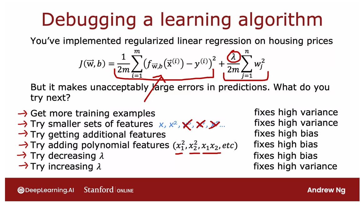
Debugging a learning algorithm

What do you try next?

High variance (Overfitting)	High bias (Underfitting)
Get more training examples	Try getting additional features
Try smaller sets of features	Try adding polynomial features
Try increasing $\lambda$	Try decreasing $\lambda$

I realized that this was a
lot of stuff on this slide.

But the takeaways I
hope you have are, if you find that your
algorithm has high variance, then the two main
ways to fix that are; either get more training
data or simplify your model.

By simplifying model I mean, either get a smaller
set of features or increase the regularization
parameter Lambda.

Your algorithm has less
flexibility to fit very complex, very
wiggly curves.

Conversely, if your
algorithm has high bias, then that means is not doing well even on
the training set.

If that’s the case,
the main fixes are to make your model more powerful or to give them
more flexibility to fit more complex or
more with me functions.

Some ways to do
that are to give it additional features or add
these polynomial features, or to decrease the
regularization parameter Lambda.

Anyway, in case you’re
wondering if you should fix high bias by
reducing the training set size, that doesn’t actually help. If you reduce the
training set size, you will fit the
training set better, but that tends to worsen your cross-validation error and the performance of your
learning algorithm, so don’t randomly throw away training examples just to try
to fix a high bias problem.

One of my PhD students
from Stanford, many years after he’d already
graduated from Stanford, once said to me that while
he was studying at Stanford, he learned about bias
and variance and felt like he got it,
he understood it.

Bias and variance is one of those concepts that takes a short time to learn, but takes a lifetime to master.

But that subsequently, after many years of work experience in a few different companies, he realized that bias
and variance is one of those concepts that takes
a short time to learn, but takes a lifetime to master.

Those were his exact words.

Bias and variance is one of
those very powerful ideas.

When I’m training
learning algorithms, I almost always try to figure out if it is high bias
or high variance.

But the way you go
about addressing that systematically is something that you will keep on getting better at through
repeated practice.

But you’ll find that understanding these ideas
will help you be much more effective at how
you decide what to try next when developing
a learning algorithm.

Now, I know that
we did go through a lot in this video
and if you feel like, boy, this isn’t lost stuff here, is okay, don’t worry about it.

Later this week in the practice labs and
practice quizzes will have also additional
opportunities to go over these ideas so that you can
get additional practice.

We’re thinking about bias and variance of different
learning algorithms.

If it seems like a lot
right now is okay, you get to practice these
ideas later this week and hopefully deepened
your understanding of them at that time.

Before moving on, bias and variance
also are very useful when thinking about how to
train a neural network. In the next video, let’s take a look
at these concepts applied to neural
network training. Let’s go on to the next video.

Bias/variance and neural networks

Was seen that high bias or
high variance are both bad in the sense that they hurt
the performance of your algorithm.

One of the reasons that neural networks
have been so successful is because your networks, together with the idea of big
data or hopefully having large data sets.

It’s given us a new way of new ways to
address both high bias and high variance. Let’s take a look.

You saw that if you’re fitting different
order polynomial is to a data set, then if you were to fit a linear
model like this on the left.

You have a pretty simple model that
can have high bias whereas you were to fit a complex model,
then you might suffer from high variance.

And there’s this tradeoff between bias and
variance, and in our example it was choosing a second order polynomial
that helps you make a tradeoff and pick a model with lowest
possible cross validation error.

And so before the days of neural networks, machine learning engineers talked a lot
about this bias variance tradeoff in which you have to balance the complexity
that is the degree of polynomial.

Or the regularization parameter
longer to make bias and variance both not be too high.

And if you hear machine learning engineers
talk about the bias variance tradeoff. This is what they’re referring to
where if you have too simple a model, you have high bias,
too complex a model high variance.

And you have to find a tradeoff between
these two bad things to find probably the best possible outcome.

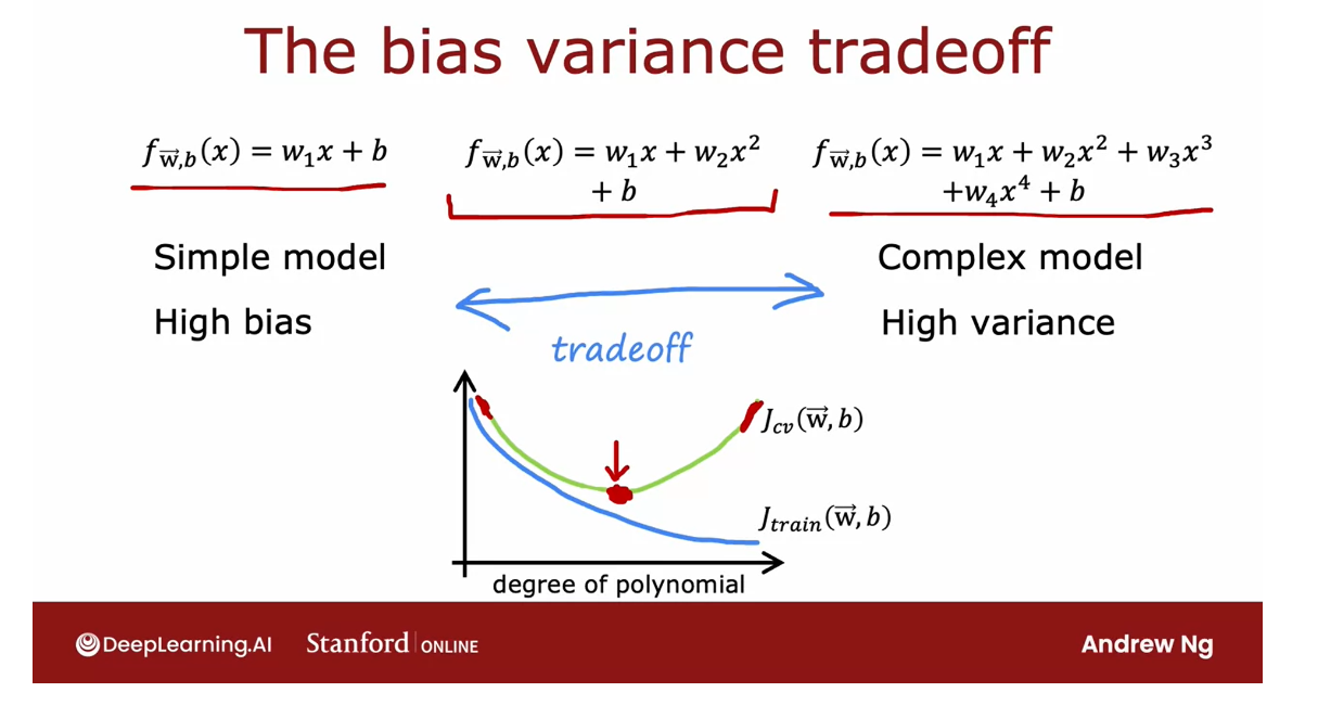
But it turns out that your networks
offer us away all of this dilemma of having to tradeoff bias and
variance with some caveats.

And it turns out that large
neural networks when trained on small term moderate sized
datasets are low bias machines.

And what I mean by that is, if you
make your neural network large enough, you can almost always fit
your training set well. So long as your training
set is not enormous.

And what this means is this gives us a new recipe to try to reduce bias or reduce variance as needed without needing to really trade off between the two of them.

And what this means is this gives us a new
recipe to try to reduce bias or reduce variance as needed without needing to
really trade off between the two of them.

So let me share with you a simple
recipe that isn’t always applicable.

But if it supplies can be very
powerful for getting an accurate model using a neural network which is
first train your algorithm on your training set and then asked does
it do well on the training set.

So measure Jtrain and
see if it is high and by high, I mean for example, relative to human
level performance or some baseline level of performance and
if it is not doing well then you have a high bias problem,
high trains error.

And one way to reduce bias is to
just use a bigger neural network and by bigger neural network, I mean either more hidden layers or
more hidden units per layer.

And you can then keep on
going through this loop and make your neural network bigger and bigger
until it does well on the training set.

Meaning that achieves the level of error
in your training set that is roughly comparable to the target level
of error you hope to get to, which could be human level performance.

After it does fall on the training set,
so the answer to that question is yes. You then ask doesn’t do well
on the trans validation set.

In other words, does it have high
variance and if the answer is no, then you can conclude that the algorithm
has high variance because it doesn’t want to train set does not
do on the cross validation set.

So that big gap in Jcv and
Jtrain indicates you probably have a high variance problem, and
if you have a high variance problem, then one way to try to fix
it is to get more data.

To get more data and go back and
retrain the model and just double-check, do you just want the training set?

If not, have a bigger network, or it does see if it does when the cross
foundation set and if not get more data.

And if you can keep on going around and
around and around this loop until eventually it
does well in the cross validation set.

Then you’re probably done because now you
have a model that does well on the cross validation set and hopefully will also
generalize to new examples as well.

Large NN: at some point it does get computationally expensive.

Now, of course there are limitations of
the application of this recipe training bigger neural network
doesn’t reduce bias but at some point it does get
computationally expensive.

That’s why the rise of neural networks
has been really assisted by the rise of very fast computers, including especially
GPUs or graphics processing units.

Hardware traditionally used to
speed up computer graphics, but it turns out has been very useful for
speeding on neural networks as well.

But even with hardware accelerators
beyond a certain point, the neural networks are so large, it takes
so long to train, it becomes infeasible.

And then of course the other
limitation is more data.

Sometimes you can only get so
much data, and beyond a certain point it’s
hard to get much more data.

The rise of deep learning

But I think this recipe explains a lot
of the rise of deep learning in the last several years, which is for applications
where you do have access to a lot of data.

Then being able to train large
neural networks allows you to eventually get pretty good
performance on a lot of applications.

One thing that was implicit in this slide
that may not have been obvious is that as you’re developing a learning algorithm,
sometimes you find that you have high bias, in which case you do things
like increase your neural network.

But then after you increase your neural
network you may find that you have high variance, in which case you might do
other things like collect more data.

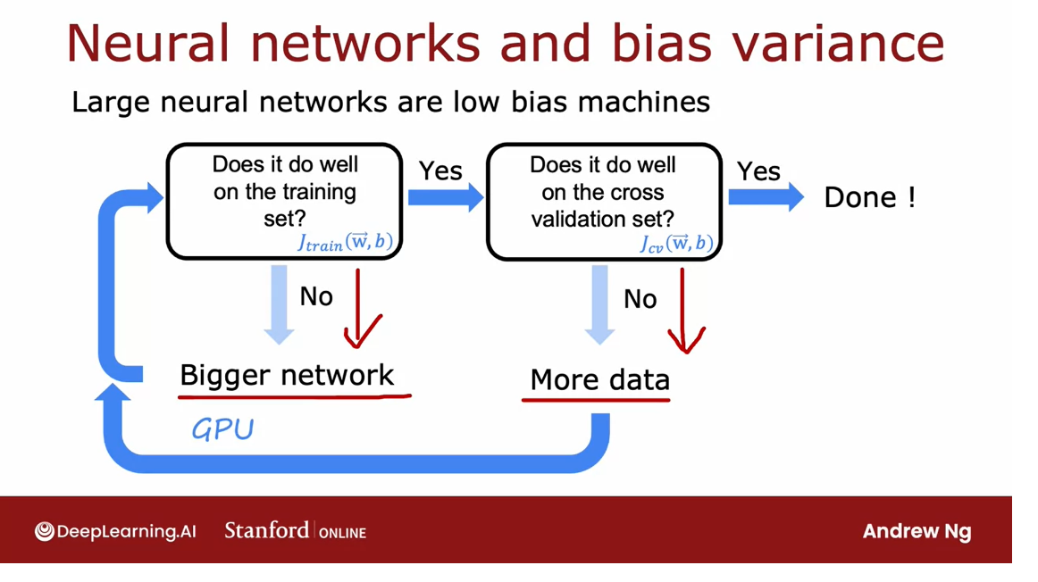
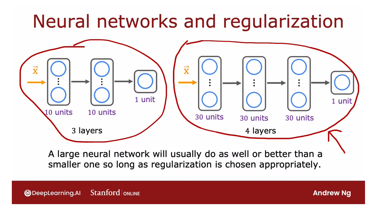
And during the hours or days or weeks,
you’re developing a machine learning algorithm at different points,
you may have high bias or high variance.

And it can change but it’s depending on
whether your algorithm has high bias or high variance at that time.

Then that can help give guidance for
what you should be trying next.

When you train your neural your network,
one thing that people have asked me before is, hey Andrew,
what if my neural network is too big?

Will that create a high variance problem?

a large neural network with well-chosen regularization, well usually do as well or better than a smaller one.

It turns out that a large neural network
with well-chosen regularization, well usually do as well or
better than a smaller one.

And so for example, if you have
a small neural network like this, and you were to switch to a much
larger neural network like this, you would think that the risk of
overfitting goes up significantly.

But it turns out that if you were to
regularize this larger neural network appropriately, then this larger neural
network usually will do at least as well or better than the smaller one.

So long as the regularization
has chosen appropriately.

So another way of saying this is that
it almost never hurts to go to launch a neural network so long as you
regularized appropriately with one caveat, which is that when you train
the larger neural network, it does become more
computational e expensive.

So the main way it hurts,
it will slow down your training and your inference process and very briefly
to regularize a neural network. T

his is what you do if
the cost function for your neural network is
the average loss and so the last year could be squared error or
logistic loss.

Then the regularization term for a neural
network looks like pretty much what you’d expect is longer over two m times
the sum of w squared where this is a sum over always W in the neural
network and similar to regularization for linear regression and logistic regression, we usually don’t regularize the parameters
be in the neural network although in practice it makes very little
difference whether you do so or not.

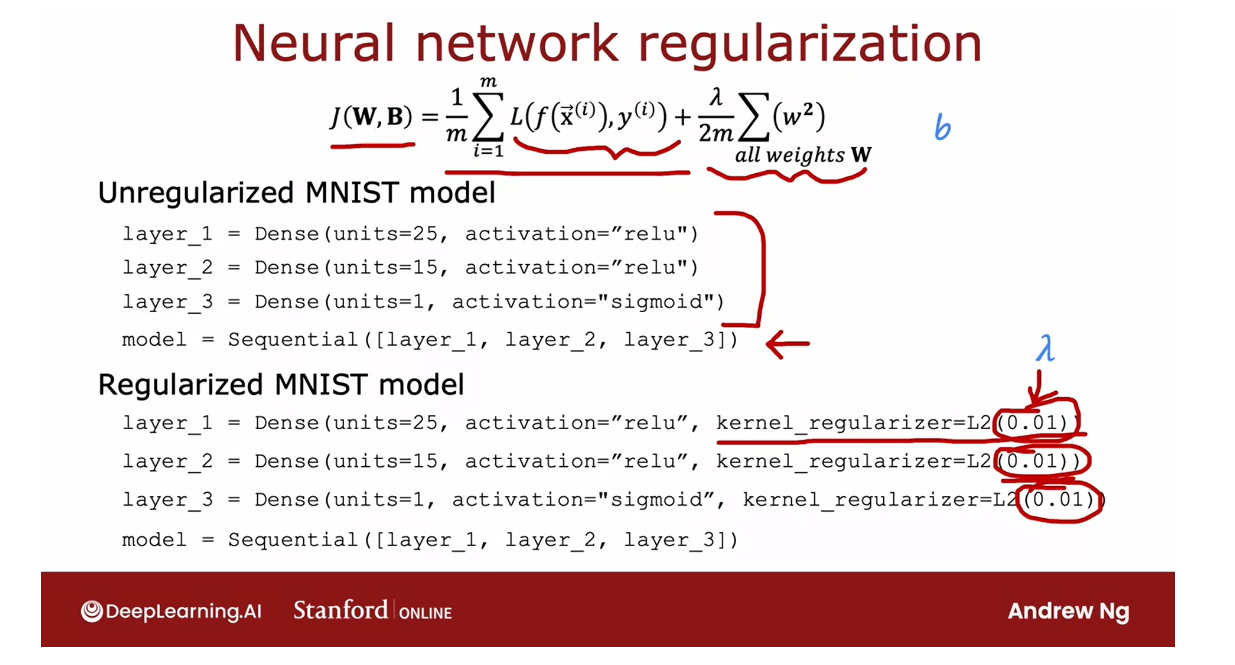
And the way you would implement
regularization in tensorflow is recall that this was the code for implementing an unregulated Rised
handwritten digit classification model.

We create three layers like so with
a number of fitting units activation And then create a sequential
model with the three layers.

If you want to add regularization
then you would just add this extra term colonel regularize A equals l. two and then 0.01 where that’s the value
of longer in terms of though actually lets you choose different values of
lambda for different layers although for simplicity you can choose the same
value of lambda for all the weights and all of the different layers as follows.

And then this will allow you to implement
regularization in your neural network.

Two takeaways

So to summarize two Takeaways,
I hope you have from this video are one.

It hardly ever hurts to have
a larger neural network so long as you regularize appropriately. one caveat being that having a larger
new network can slow down your speed.

So maybe that’s the one way it hurts, but
it shouldn’t hurt your algorithm performance for the most part and in fact it
could even help it significantly.

And second so
long as your training set isn’t too large.

Then a new network, especially large neural network
is often a low bias machine.

It just fits very complicated functions
very well, which is why when I’m training neural networks, I find that I’m often
fighting various problems rather than bias problems, at least if the neural
network is large enough.

So the rise of deep learning has really
changed the way that machine learning practitioners think about bias and
variance.

Having said that even when you’re training
a neural network measuring bias and variance and using that to God, what you do next
is often a very helpful thing to do. So that’s it for bias and variance.

Let’s go on to the next video. We will take all the ideas
we’ve learned and see how they fit in to the development
process of machine learning systems. And I hope that we’ll tie a lot of these
pieces together to give you practical advice for how to quickly move forward
in the development of your machine learning systems

[4] Practice quiz: Bias and variance

Practice quiz: Bias and variance

Latest Submission Grade 100%

Question 1

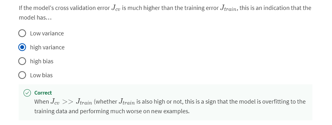
When $J_{cv}>>J_{train}$ (whether $J_{train}$is also high or not, this is a sign that the model is overfitting to the training data and performing much worse on new examples.

Question 2

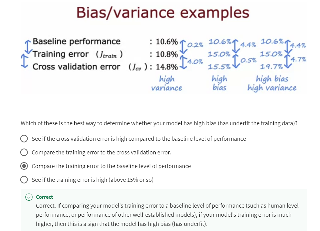
Correct. If comparing your model’s training error to a baseline level of performance (such as human level performance, or performance of other well-established models), if your model’s training error is much higher, then this is a sign that the model has high bias (has underfit).

Question 3

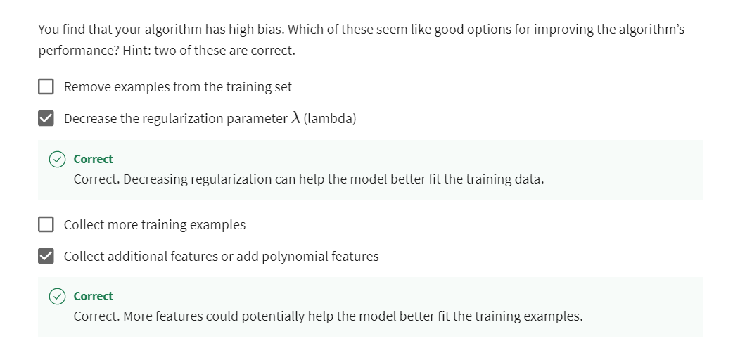
Question 4

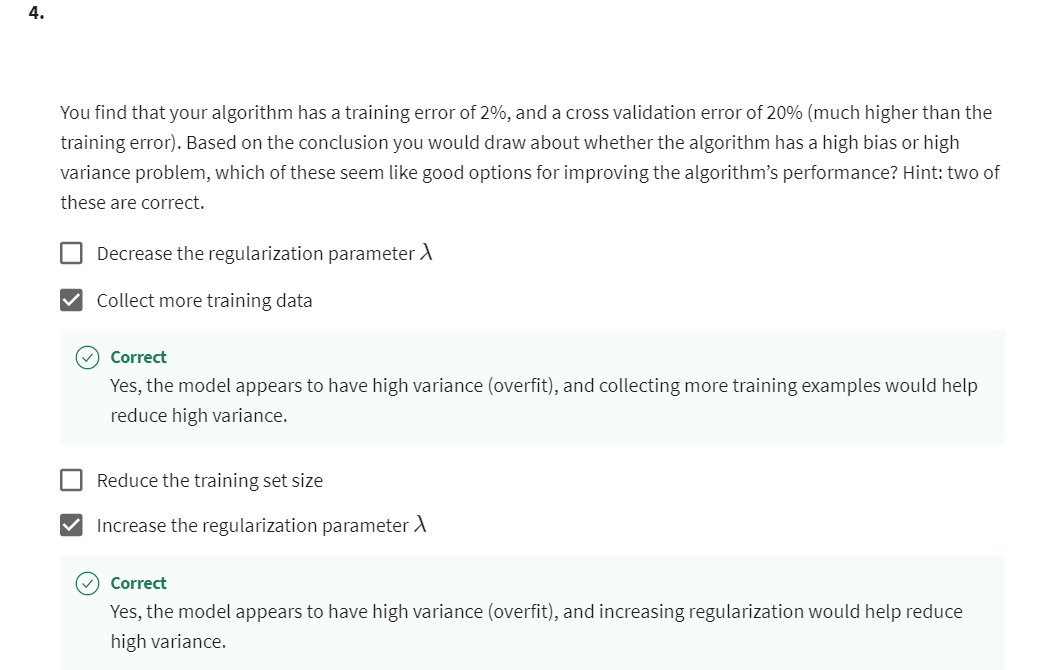
[5] Machine learning development process

Iterative loop of ML development

In the next few videos, I’d like to share
with you what is like to go through the process of developing a machine
learning system so that when you are
doing so yourself, hopefully, you’d
be in a position to make great decisions at many stages of the machine
learning development process.

Let’s take a look first at the iterative loop of machine
learning development.

This is what developing a machine learning model
will often feel like.

First, you decide on what is the overall architecture
of your system. That means choosing your
machine learning model as well as deciding
what data to use, maybe picking the
hyperparameters, and so on.

Then, given those decisions, you would implement
and train a model.

As I’ve mentioned before, when you train a model
for the first time, it will almost never work
as well as you want it to.

The next step that
I recommend then is to implement or to look
at a few diagnostics, such as looking at the bias and variance of your
algorithm as well as something we’ll see in the next video called
error analysis.

Based on the insights
from the diagnostics, you can then make decisions like do want to make
your neural network bigger or change the Lambda
regularization parameter, or maybe add more data or add more features
or subtract features.

Take multiple iterations through the loop

Then you go around this loop again with your new
choice of architecture, and it will often take
multiple iterations through this loop until you get to the
performance that you want.

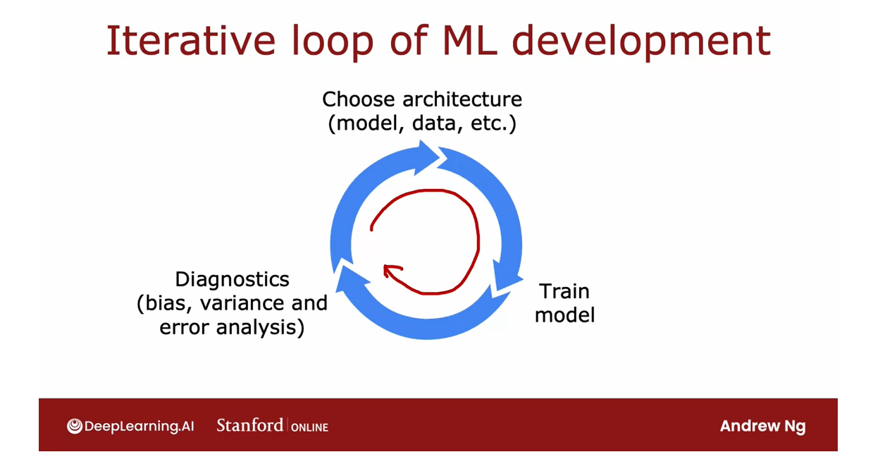
Let’s look at an
example of building an email spam classifier.

I think many of us
passionately hate email spam and this
is a problem that I worked on years ago and
also was involved in starting an anti-spam
conference once years ago.

The example on the left is what a highly spammy email
might look like. Deal of the week, by
now, Rolex watches. Spammers will
sometimes deliberately misspell words like these, watches, medicine, and mortgages in order to try to trip
up a spam recognizer.

In contrast, this email on the right is an
actual email I once got from my younger
brother Alfred about getting together
for Christmas.

How do you build a classifier to recognize spam
versus non-spam emails?

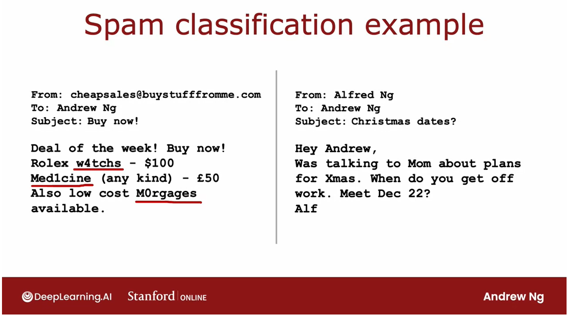
One way to do so
would be to train a supervised learning algorithm where the input features x will be the features of an email and the
output label y will be one or zero depending on whether
it’s spam or non-spam.

This application is an example of text classification
because you’re taking a text document
that is an email and trying to classify it
as either spam or non-spam.

One way to construct the features of the
email would be to say, take the top 10,000 words in
the English language or in some other dictionary
and use them to define features x_1, x_2
through x_10,000.

For example, given this
email on the right, if the list of
words we have is a, Andrew buy deal
discount and so on. Then given the
email on the right, we would set these
features to be, say, 0 or 1, depending on whether
or not that word appears.

The word a does not appear. The word Andrew does appear. The word buy does
appear, deal does, discount does not, and so on, and so you can construct
10,000 features of this email.

There are many ways to
construct a feature vector.

Another way would be to let these numbers
not just be 1 or 0, but actually, count
the number of times a given word
appears in the email. If buy appears twice, maybe you want to set this to 2, but setting into just 1 or 0. It actually works decently well.

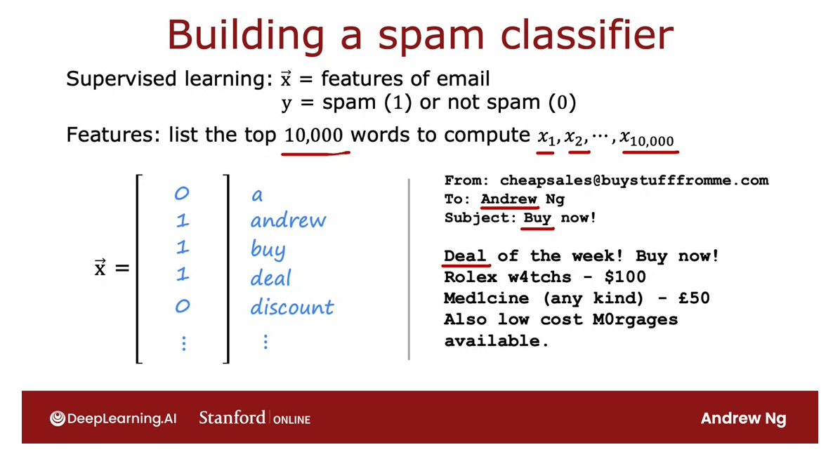
Given these features,
you can then train a classification
algorithm such as a logistic regression model
or a neural network to predict y given
these features x.

After you’ve trained
your initial model, if it doesn’t work
as well as you wish, you will quite likely have multiple ideas for improving the learning algorithm’s
performance.

For example, is always
tempting to collect more data.

In fact, I have friends
that have worked on very large-scale
honeypot projects.

These are projects that
create a large number of fake email
addresses and tries to deliberately to get these
fake email addresses into the hands of spammers
so that when they send spam email to these fake
emails well we know these are spam email messages
and so this is a way to get a lot of spam data.

Or you might decide
to work on developing more sophisticated features
based on the email routing.

Email routing refers to the
sequence of compute service. Sometimes around the
world that the email has gone through all
this way to reach you and emails actually have what’s called email
header information.

That is information
that keeps track of how the email has traveled
across different servers, across different networks
to find its way to you. Sometimes the path that
an email has traveled can help tell you if it was
sent by a spammer or not.

Or you might work
on coming up with more sophisticated features from the email body that is
the text of the email. In the features I
talked about last time, discounting and discount may be treated as different words, and maybe they should be
treated as the same words.

Or you might decide to
come up with algorithms to detect misspellings or deliberate misspellings
like watches, medicine, and mortgage and this too could help you decide
if an email is spammy.

Given all of these and
possibly even more ideas, how can you decide which of these ideas are more
promising to work on?

Because choosing the
more promising path forward can speed
up your project easily 10 times compared
to if you were to somehow choose some of the
less promising directions.

For example, we’ve
already seen that if your algorithm has high bias
rather than high variance, then spending months
and months on a honeypot project may not be the most
fruitful direction.

But if your algorithm
has high variance, then collecting more
data could help a lot.

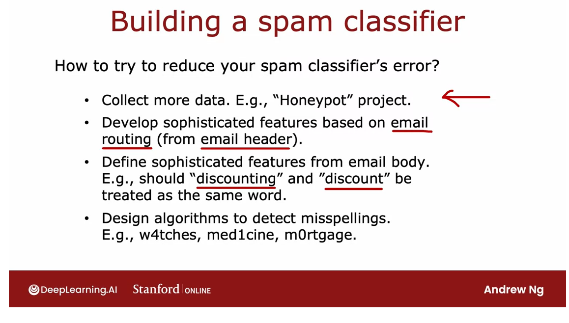
Doing the iterative loop of
machinery and development, you may have many
ideas for how to modify the model or the data, and it will be coming up with different diagnostics
that could give you a lot of guidance on what choices
for the model or data, or other parts of the architecture could be
most promising to try.

In the last several videos, we’ve already talked
about bias and variance.

In the next video,
I’d like to start describing to you the
error analysis process, which has a second key
set of ideas for gaining insight about what architecture choices
might be fruitful. That’s the iterative
loop of machine learning development and
using the example of building a spam classifier. Let’s take a look at what
error analysis looks like. Let’s do that in the next video.

Error analysis

In terms of the
most important ways to help you run diagnostics to choose what to try next to improve your learning
algorithm performance, I would say bias and
variance is probably the most important idea and error analysis would probably
be second on my list.

Let’s take a look
at what this means.

Concretely, let’s say
you have m_cv equals 500 cross validation
examples and your algorithm misclassifies 100 of these 500 cross
validation examples.

The error analysis process just refers to manually
looking through these 100 examples and trying to gain insights into where the
algorithm is going wrong.

Try to group the misclassified examples into common themes or common properties or common traits.

Specifically, what I
will often do is find a set of examples that
the algorithm has misclassified examples from
the cross validation set and try to group them into common themes or common
properties or common traits.

For example, if you notice
that quite a lot of the misclassified spam emails
are pharmaceutical sales, trying to sell
medicines or drugs then I will actually go through
these examples and counter by hand how many
emails in this classified are pharmaceutical
spam and say there are 21 emails that are
pharmaceutical spam.

Or if you suspect that deliberate misspellings may be tripping over your spam classifier then I will also go through and just
count up how many of these examples that it misclassified had a
deliberate misspelling.

Let’s say I find
three out of a 100.

Or looking through the email routing info I find seven has unusual email routing and 18 emails trying to steal
passwords or phishing emails.

Spam is sometimes also, instead of writing
the spam message in the email body they
instead create an image and then writes to spam the message inside an image
that appears in the email.

This makes it a
little bit harder for learning algorithm to
figure out what’s going on.

Maybe some of those emails are
these embedded image spam.

If you end up with
these counts then that tells you that
pharmaceutical spam and emails trying to steal passwords or phishing
emails seem to be huge problems whereas
deliberate misspellings, well, it is a problem
it is a smaller one.

In particular, what this
analysis tells you is that even if you were to build really sophisticated
algorithms to find deliberate
misspellings it will only solve three out of 100 of
your misclassified examples.

The net impact seems like
it may not be that large. Doesn’t mean it’s
not worth doing?

But when you’re
prioritizing what to do, you might therefore decide not to prioritizes this as highly.

By the way, I’m
telling the story because I once actually
spent a lot of time building algorithms to find
deliberate misspellings and spam emails only much later to realize that the net impact
was actually quite small.

This is one example where I wish I’d done more
careful error analysis before spending a lot of time myself trying to find these
deliberate misspellings.

Just a couple of notes
on this process.

These categories can be overlapping or in other words they’re not mutually exclusive.

For example, there can be a pharmaceutical spam email
that also has unusual routing or a password that has
deliberate misspellings and is also trying to carry
out the phishing attack.

One email can be counted
in multiple categories.

In this example, I had
said that the algorithm is classified as 100
examples and we’ll look at all 100 examples manually.

If you have a larger
cross validation set, say we had 5,000 cross validation examples
and if the algorithm misclassified say 1,000 of
them then you may not have the time depending
on the team size and how much time you have
to work on this project.

Sample randomly a subset of all the examples

You may not have the
time to manually look at all 1,000 examples that the
algorithm is classifies.

In that case, I
will often sample randomly a subset of
usually around a 100, maybe a couple 100
examples because that’s the amount that you can look through in a reasonable
amount of time.

Hopefully looking
through maybe around a 100 examples will give
you enough statistics about whether the most common
types of errors and therefore where maybe most fruitful to focus
your attention.

After this analysis, if you
find that a lot of errors are pharmaceutical spam emails
then this might give you some ideas or inspiration
for things to do next.

For example, you may decide to collect more data but not
more data of everything, but just try to find more data of pharmaceutical spam emails so that the learning algorithm
can do a better job recognizing these
pharmaceutical spam.

Or you may decide
to come up with some new features that are
related to say specific names of drugs or specific names of pharmaceutical products of the standards you’re
trying to sell in order to help your
learning algorithm become better at recognizing
this type of former spam.

Then again this might
inspire you to make specific changes
to the algorithm relating to detecting
phishing emails.

For example, you might look at the URLs in the
email and write special code to come
with extra features to see if it’s linking
to suspicious URLs.

Or again, you might
decide to get more data of phishing emails specifically in order to help your learning algorithm do a better job of recognizing them.

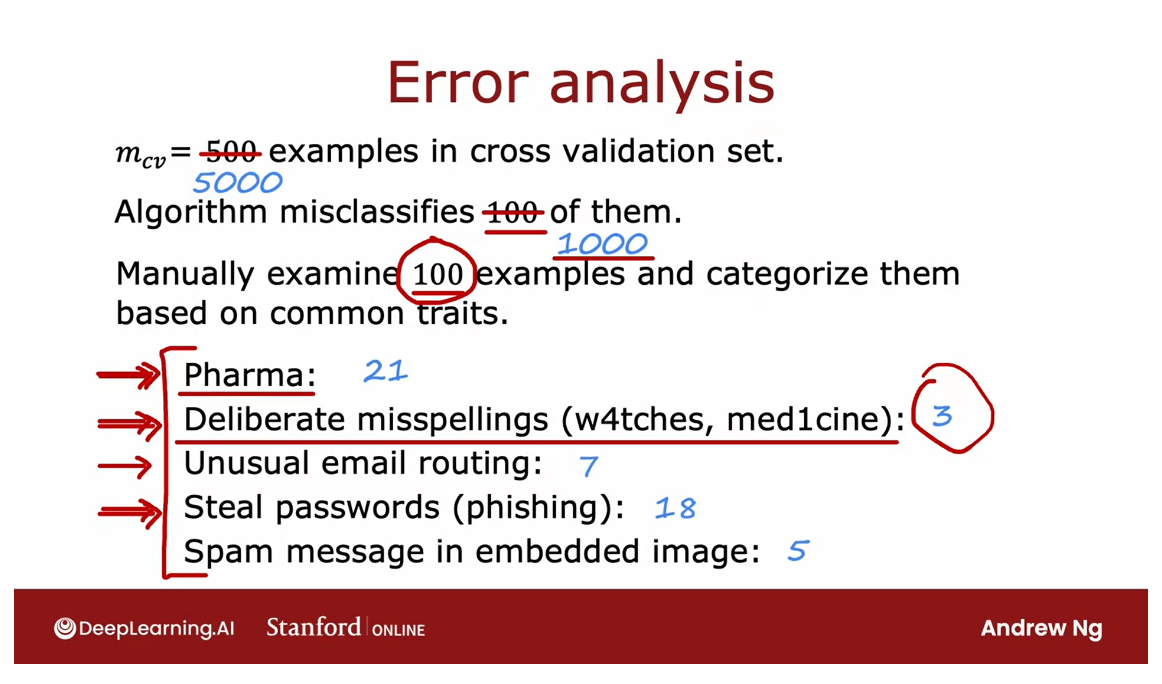
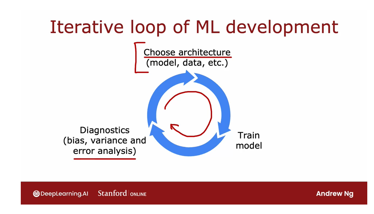
The point of this error analysis is by manually examining a set of examples that your algorithm is misclassifying or mislabeling.

The point of this error analysis
is by manually examining a set of examples
that your algorithm is misclassifying
or mislabeling.

Often this will create inspiration for what might
be useful to trying it and sometimes it can also tell
you that certain types of errors are sufficiently
rare that they aren’t worth as much of
your time to try to fix.

Returning to this list, a bias variance
analysis should tell you if collecting more
data is helpful or not.

Based on our error analysis in the example
Lisa went through, it looks like more
sophisticated email features could help but
only a bit whereas more sophisticated
features to detect former spam or phishing
emails could help a lot.

These detecting
misspellings would not help nearly as much.

In general I found both the bias variance diagnostic as well as carrying out this form of error analysis to be really helpful to screening or to deciding which changes to the model are more promising to try on next.

In general I found both the bias variance diagnostic as well as carrying out this form
of error analysis to be really helpful
to screening or to deciding which changes to the model are more
promising to try on next.

Now one limitation of error
analysis is that it’s much easier to do for problems
that humans are good at.

You can look at the email and say you think
is a spam email, why did the average
get it wrong?

Error analysis can be a bit harder for tasks that even humans aren’t good at.

Error analysis can
be a bit harder for tasks that even
humans aren’t good at.

For example, if you’re
trying to predict what ads someone will
click on on the website.

Well, I can’t predict what
someone will click on.

Error analysis there actually
tends to be more difficult.

But when you apply
error analysis to problems that you can it can be extremely helpful for focusing attention on the
more promising things to try.

That in turn can easily save you months of otherwise
fruitless work.

In the next video, I’d like to dive deeper into
the problem of adding data. When you train a
learning algorithm, sometimes you decide there’s high variance and you want
to get more data for it.

Some techniques they
can make how you add data much more efficient. Let’s take a look at that so that hopefully
you’ll be armed with some good ways to get more data for your
learning application.

Adding data

In this video,
I’d like to share with you some tips for adding data or collecting more data or
sometimes even creating more data for your machine learning application.

Just a heads up that this in the next few
videos will seem a little bit like a grab bag of different techniques.

And I apologize if it seems
a little bit grab baggy and that’s because machine learning
applications are different.

Machine learning is applied to so
many different problems and for some humans are great at creating labels.

And for some you can get more data and
for some you can’t.

And that’s why different applications
actually sometimes call for slightly different techniques.

But I hope in this in the next few videos
to share with you some of the techniques that are found to be most useful for
different applications, although not every one of them will
apply for every single application.

But I hope many of them
would be useful for many of the applications that
you’ll be working on as well.

Some tips for how to add data for your application

But let’s take a look at some tips for
how to add data for your application.

focus on adding more data of the types where analysis has indicated it might help.

When training machine learning algorithms, it feels like always we wish we had
even more data almost all the time.

And so sometimes it’s tempting to let’s
just get more data of everything.

But, trying to get more data of all
types can be slow and expensive.

Instead, an alternative way of adding
data might be to focus on adding more data of the types where analysis
has indicated it might help.

In the previous slide we saw if
error analysis reviewed that farmer stamp was a large problem,
then you may decide to have a more targeted effort not to get more
data everything under the sun but to stay focused on getting
more examples of farmer stamp.

And with a more modest cost this
could let you add just the emails you need to hope you’re learning and
get smarter on recognizing pharma spam.

And so
one example of how you might do this is, if you have a lot of unlabeled email data,
say emails sitting around and no one has bothered to label yet
a stamp or non stamp.

You might be able to go
to the unlabeled data.

You may able to ask your labors to quickly
skim through the unlabeled data and find more examples specifically
a farmer related spam.

And this could boost your learning
algorithm performance much more than just trying to add more data
of all sorts of emails.

But the more general pattern I
hope you take away from this is, if you have some ways to add more
data of everything that’s okay.

Nothing wrong with that.

But if error analysis has indicated
that there are certain subsets of the data that the algorithm is
doing particularly poorly on.

And that you want to
improve performance on, then getting more data of just the types
where you wanted to do better.

Be it more examples of
pharmaceutical spam or more examples of phishing spam or
something else.

That could be a more efficient way
to add just a little bit of data but boost your algorithms
performance by quite a lot.

Data augmentation: Take an existing training example to create a new training example

Beyond getting your hands on
brand new training examples xy.

There’s another technique that’s why
they use especially for images and audio data that can increase your
training set size significantly.

This technique is called
data augmentation.

And what we’re going to do is take
an existing train example to create a new training example.

For example if you’re trying to
recognize the letters from A to Z for an [INAUDIBLE] optical
character recognition problem.

So not just the digits 0-9 but
also the letters from A to Z.

Given an image like this,
you might decide to create a new training example by
rotating the image a bit.

Or by enlarging the image a bit or
by shrinking a little bit or by changing the contrast of the image.

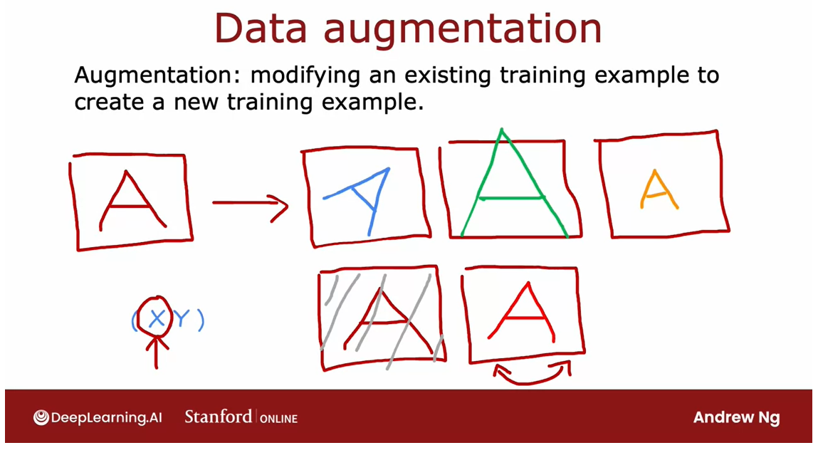
For a more advanced example
of data augmentation. You can also take the letter A and
place a grid on top of it.

And by introducing random warping of
this grid, you can take the letter A.

And introduce war pings of the leather
A to create a much richer library of examples of the letter A.

And this process of distorting these
examples then has turned one image of one example into here training
examples that you can feed to the learning algorithm to
hope it learn more robustly.

What is the letter A.

And these are examples of distortions
to the image that don’t change the fact that this is still the alphabet,
that this is still the letter A.

And for some letters but not others
you can also take the mirror image of the letter and
it still looks like the letter A.

But this only applies to some letters but these would be ways of taking
a training example X, Y.

And applying a distortion or
transformation to the input X ,in order to come up with another
example that has the same label.

And by doing this you’re telling the
algorithm that the letter A rotated a bit or enlarged a bit or shrunk a little
bit it is still the letter A.

And creating additional examples like
this holds the learning algorithm, do a better job learning how
to recognize the letter A.

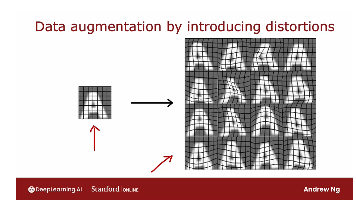
This idea of data augmentation
also works for speech recognition.

Let’s say for a voice search application, you have an original audio
clip that sounds like this. >> What is today’s weather. >>

One way you can apply
data documentation to speech data would be to take noisy
background audio like this.

For example, this is what
the sound of a crowd sounds like.

And it turns out that if you
take these two audio clips, the first one and the crowd noise and
you add them together, then you end up with an audio
clip that sounds like this. >> What is today’s weather. >>

And you just created an audio clip
that sounds like someone saying what’s the weather today.

But they’re saying it around
the noisy crowd in the background.

Or in fact if you were to take
a different background noise, say someone in the car, this is what
background noise of a car sounds like.

And you want to add the arsenal audio
clip to the car noise, then you get this. >> What is today’s weather. >> And it sounds like
the original audio clip, but as if the speaker was
saying it from a car.

And the more advanced data orientation
step would be if you make the original audio sound like you’re recording it on
a bad cell phone connection like this.

And so we’ve seen how you can take one
audio clip and turn it into three training examples here, one with crowd background
noise, one with car background noise and one as if it was recorded on
a bad cell phone connection.

And the times I worked on
speech recognition systems, this was actually a really critical
technique for increasing artificially the size of the training data I had to
build a more accurate speech recognizer.

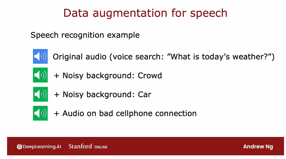
One tip for
data augmentation is that the changes or the distortions you make to the data, should be representative of the types of
noise or distortions in the test set.

So for example, if you take the letter
a and warp it like this, this still looks like examples of letters you might see out
there that you would like to recognize.

Or for audio adding background noise or
bad cellphone connection if that’s representative of what
you expect here in the test set, then this will be helpful ways to carry
out data augmentation on your audio data.

In contrast is usually not that helpful at
purely random meaningless noise to data.

For example,
you have taken the letter A and I’ve added per pixel noise
where if Xi is the intensity or the brightness of pixel i,
if I were to just add noise to each pixel, they end up with images
that look like this.

But if to the extent that this isn’t
that representative of what you see in the test set because you don’t often
get images like this in the test set is actually going to be less helpful.

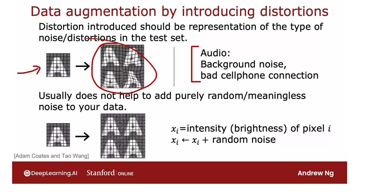
So one way to think about data
augmentation is how can you modify or warp or distort or
make more noise in your data.

But in a way so that what you get is still quite similar
to what you have in your test set, because that’s what the learning algorithm
will ultimately end up doing well on.

Data synthesis: create brand new examples

Now, whereas data augmentation takes
an existing training example and modifies it to create
another training example.

There’s one of the techniques which is
data synthesis in which you make up brand new examples from scratch.

Not by modifying an existing example but
by creating brand new examples.

So take the example of photo OCR.

Photo OCR or photo optical
character recognition refers to the problem of looking at
an image like this and automatically having a computer read
the text that appears in this image.

So there’s a lot of text in this image. How can you train in OCR algorithm to
read text from an image like this?

Well, when you look closely at what
the letters in this image looks like they actually look like this.

So this is real data
from a photo OCR task. And one key step with the photo OCR task
is to be able to look at the little image like this, and
recognize the letter at the middle.

So this has T in the middle,
this has the letter L in the middle, this has the letter C in the middle and
so on.

So one way to create artificial data for
this task is if you go to your computer’s text editor,
you find that it has a lot of different fonts and
what you can do is take these fonds and basically type of random
text in your text editor.

And screenshotted using different
colors and different contrasts and very different fonts and you get
synthetic data like that on the right.

The images on the left were real data from
real pictures taken out in the world.

The images on the right are synthetically
generated using fonds on the computer, and it actually looks pretty realistic.

So with synthetic data generation
like this you can generate a very large number of images or
examples for your photo OCR task.

It can be a lot of work to write
the code to generate realistic looking synthetic data for a given application.

But when you spend the time to do so, it can sometimes help you generate
a very large amount of data for your application and give you a huge
boost to your algorithms performance.

Synthetic data generation has
been used most probably for computer vision toss and
less for other applications.

Not that much for audio talks as well.

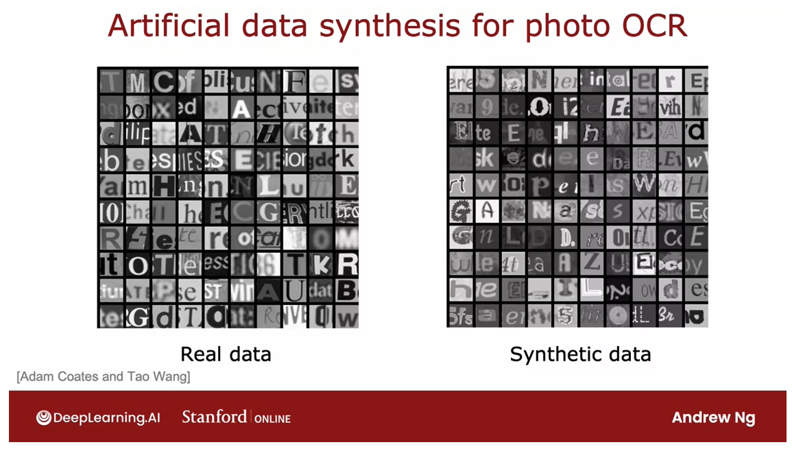
engineering your data 设计数据

engineer: 密谋策划;设计制造;改变…的基因(或遗传)结构

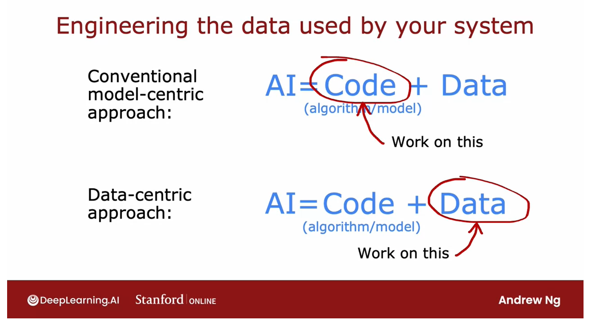
All the techniques you’ve
seen in this video related to finding ways to engineer
the data used by your system.

In the way that machine learning has
developed over the last several decades, many decades.

Most machine learning researchers
attention was on the conventional model centric approach and here’s what I mean.

A machine learning system or an AI system
includes both code to implement your algorithm or your model, as well as the data
that you train the algorithm model.

and over the last few decades,
most researchers doing machine learning research would download the data set and
hold the data fixed while they focus on improving the code or
the algorithm or the model.

Thanks to that paradigm of
machine learning research.

I find that today the algorithm we have
access to such as linear regression, the district Grecian neural networks also
decision trees we should see next week.

There are algorithms that
already very good and will work well for many applications.

And so sometimes it can be more
fruitful to spend more of your time taking a data centric
approach in which you focus on engineering the data
used by your algorithm.

And this can be anything from collecting
more data just on pharmaceutical spam. If that’s what error
analysis told you to do.

To using data augmentation to
generate more images or more audio or using data synthesis to just
create more training examples.

And sometimes that focus on the data can
be an efficient way to help your learning algorithm improve its performance.

So I hope that this video gives you
a set of tools to be efficient and effective in how you add more data to get
your learning algorithm to work better.

Now there are also some applications where
you just don’t have that much data and it’s really hard to get more data.

It turns out that there’s a technique
called transfer learning which could apply in that setting to give your learning
algorithm performance a huge boost.

And the key idea is to take data from
a totally different barely related tasks.

But using a neural network there’s
sometimes ways to use that data from a very different tasks to get your
algorithm to do better on your application. Doesn’t apply to everything, but
when it does it can be very powerful. Let’s take a look in the next video and
how transfer learning works.

Transfer learning: using data from a different task

When you don’t have that much data, transfer learning is a wonderful technique that lets you use data from a different task to help on you application.

For an application where you
don’t have that much data, transfer learning is a wonderful technique
that lets you use data from a different task
to help on your application.

This is one of those
techniques that I use very frequently.

Let’s take a look at how
transfer learning works.

Here’s how transfer
learning works.

Let’s say you want to recognize the handwritten digits from zero through nine
but you don’t have that much labeled data of
these handwritten digits.

Here’s what you can do.

Say you find a very large datasets of one million images
of pictures of cats, dogs, cars, people, and so
on, a thousand classes.

You can then start by training a neural network on
this large dataset of a million images with a
thousand different classes and train the algorithm to
take as input an image X, and learn to recognize any of these 1,000 different classes.

In this process, you end up learning parameters
for the first layer of the neural network W^1, b^1, for the second layer W^2, b^2, and so on, W^3, b^3, W^4, b^4, and W^5,
b^5 for the output layer.

To apply transfer learning, what you do is then
make a copy of this neural network where you would chip the parameters W^1, b^1, W^2, b^2, W^3, b^3, and W^4, b^4.

But for the last layer, you would eliminate the output
layer and replace it with a much smaller output
layer with just 10 rather than 1,000 output units.

These 10 output units will correspond to the classes zero, one, through nine that you want your neural
network to recognize.

Notice that the parameters W^5, b^5 they can’t be copied over because the dimension of
this layer has changed, so you need to come up
with new parameters W^5, b^5 that you need to train from scratch rather than just copy it from the previous
neural network.

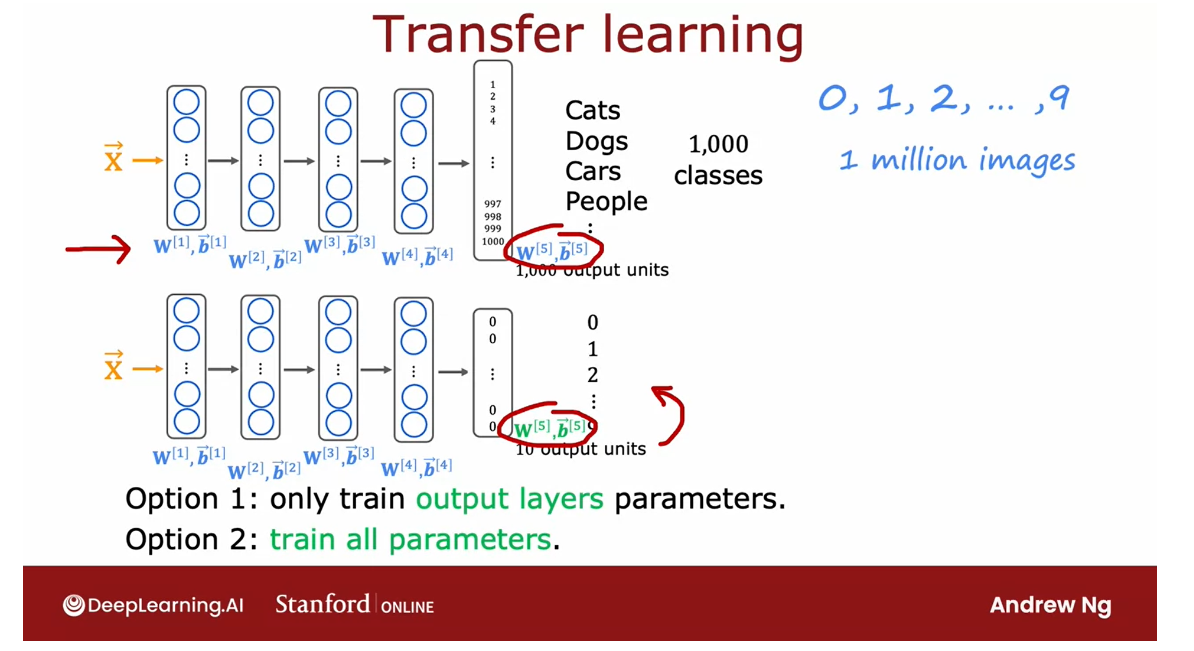
In transfer learning, what you can do is use the parameters from
the first four layers, really all the layers except
the final output layer as a starting point for the
parameters and then run an optimization algorithm
such as gradient descent or the Adam optimization
algorithm with the parameters initialized using the values from this neural
network up on top.

In detail, there are two
options for how you can train this neural
networks parameters.

Option 1

Option 1 is you only train
the output layers parameters.

Only train the output layers parameters

Hold other parameters fix and don’t even bother to change them.

You would take the
parameters W^1, b^1, W^2, b^2 through W^4, b^4 as the values
from on top and just hold them fix and don’t
even bother to change them, and use an algorithm like
Stochastic gradient descent or the Adam optimization
algorithm to only update W^5, b^5 to lower the
usual cost function that you use for learning to recognize these digits zero to nine from a small
training set of these digits zero to nine,
so this is Option 1.

Option 2

Train all the parameters

A large training set, we should select option 2

Option 2 would be to train
all the parameters in the network including
W^1, b^1, W^2, b^2 all the way through W^5, b^5 but the first four
layers parameters would be initialized using the values
that you had trained on top.

If you have a very
small training set then Option 1 might
work a little bit better, but if you have a training
set that’s a little bit larger then Option 2 might
work a little bit better.

This algorithm is called
transfer learning because the intuition is by
learning to recognize cats, dogs, cows, people, and so on.

It will hopefully, have learned some plausible
sets of parameters for the earlier layers for
processing image inputs.

Then by transferring
these parameters to the new neural network, the new neural network starts
off with the parameters in a much better place so that we have just a little
bit of further learning.

Hopefully, it can end up
at a pretty good model.

Pretrain

These two steps of
first training on a large dataset and then tuning the parameters further on a smaller dataset go by the name of supervised pre-training
for this step on top.

That’s when you train
the neural network on a very large dataset of say a million images of not
quite the related task.

Fine tune

Then the second step is called fine tuning where you take
the parameters that you had initialized or gotten from supervised pre-training and then run gradient descent further to fine tune the weights to suit the specific application of handwritten digit recognition
that you may have.

If you have a small dataset, even tens or hundreds
or thousands or just tens of thousands of images of the
handwritten digits, being able to learn from
these million images of a not quite related
task can actually help your learning algorithm’s
performance a lot.

You don’t need to be the one to carry out supervised pretraining.

One nice thing about
transfer learning as well is maybe you don’t
need to be the one to carry out
supervised pre-training.

For a lot of neural networks, there will already be
researchers they have already trained a neural
network on a large image and will have posted a trained neural networks
on the Internet, freely licensed for anyone
to download and use.

What that means is rather than carrying out the
first step yourself, you can just download the neural network that
someone else may have spent weeks training and then
replace the output layer with your own output layer and carry out either Option 1 or Option 2 to fine tune
a neural network that someone else
has already carried out supervised pre-training on, and just do a little bit
of fine tuning to quickly be able to get a neural network that performs well on your task.

Downloading a
pre-trained model that someone else has trained
and provided for free is one of those techniques
where by building on each other’s work
on machine learning community we can all get
much better results.

By the generosity of other
researchers that have pre-trained and posted their
neural networks online.

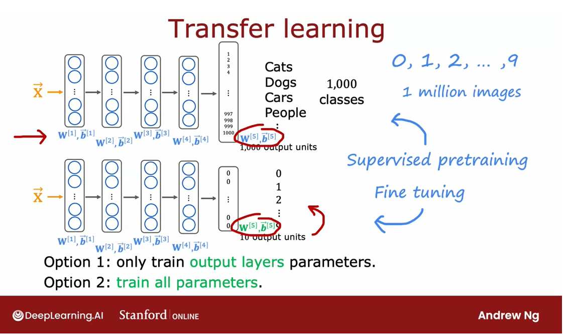
What does transfer learning work?

But why does transfer
learning even work?

How can you possibly
take parameters obtained by recognizing
cats, dogs, cars, and people and use
that to help you recognize something as different
as handwritten digits?

Here’s some intuition behind it.

Detect edges

If you are training a neural
network to detect, say, different objects from images, then the first layer of a neural network may learn to
detect edges in the image.

We think of these as
somewhat low-level features in the image which
is to detect edges.

Each of these squares is a visualization of what a
single neuron has learned to detect as learn
to group together pixels to find
edges in an image.

Detect corners

The next layer of the neural
network then learns to group together edges
to detect corners.

Each of these is a
visualization of what one neuron may
have learned to detect, must learn to technical, simple shapes like corner
like shapes like this.

Detect more complex generic shapes, basic shapes

The next layer of the
neural network may have learned to detect some
are more complex, they store generic shapes like basic curves or smaller
shapes like these.

That’s why by learning on detecting lots of
different images, you’re teaching the neural
network to detect edges, corners, and basic shapes.

That’s why by training a neural network to detect
things as diverse as cats, dogs, cars and people, you’re helping it
to learn to detect these pretty generic features of images and finding edges, corners, curves, basic shapes.

This is useful for many
other computer vision tasks, such as recognizing
handwritten digits.

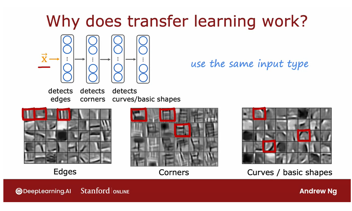
Restriction of pretraining: on the same type of input, desired dimensions

One restriction of
pre-training though, is that the image type x has to be the same for the pre-training and
fine-tuning steps.

If the final task you want to solve is a computer
vision tasks, then the pre-training
step also has been a neural network trained
on the same type of input, namely an image of the
desired dimensions.

Conversely, if your goal is to build a speech recognition
system to process audio, then a neural network
pre-trained on images probably won’t
do much good on audio.

Instead, you want
a neural network pre-trained on audio data, there you then fine tune on your own audio dataset and the same for other types
of applications.

You can pre-train a neural
network on text data and If your application has a save feature input
x of text data, then you can fine
tune that neural network on your own data.

To summarize, these are the two steps for
transfer learning.

Step 1 is download neural
network with parameters that have been pre-trained
on a large dataset with the same input type
as your application.

That input type could be
images, audio, texts, or something else, or if you don’t want to download
the neural network, maybe you can train your own.

But in practice, if
you’re using images, say, is much more common to download someone else’s
pre-trained neural network.

Then further train or fine tune the network
on your own data. I found that if you can get a neural network pre-trained
on large dataset, say a million images, then sometimes you can use
a much smaller dataset, maybe a thousand images, maybe even smaller, to fine tune the neural network
on your own data and get pretty good results.

I’d sometimes train
neural networks on as few as 50 images that were quite well
using this technique, when it has already
been pre-trained on a much larger dataset.

This technique isn’t panacea., you can’t get every application to work just on 50 images, but it does help a
lot when the dataset you have for your application
isn’t that large.

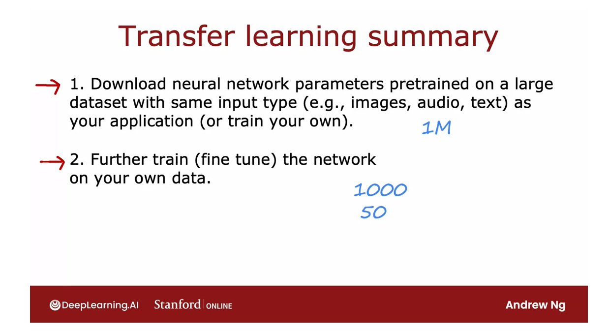
By the way, if you’ve heard of advanced techniques
in the news like GPT-3 or BERTs or neural networks
pre-trained on ImageNet, those are actually examples of neural networks
that they have someone else’s pre-trained on a
very large image datasets or text dataset, they can then be fine tuned
on other applications.

If you haven’t heard of GPT-3, or BERTs, or ImageNet, don’t worry about it,
whether you have.

Those have been
successful applications of pre-training in the
machine learning literature.

\If you haven’t heard of GPT-3, or BERTs, or ImageNet,
don’t worry about it, but if you have, those have been successful applications
of transfer learning in the machine
learning literature.

One of the things I like about transfer learning
is just that one of the ways that the machine
learning community has shared ideas, and code, and even parameters, with each other
because thanks to the researchers that
have pre-trained large neural networks and
posted the parameters on the internet freely for anyone
else to download and use.

This empowers anyone
to take models, their pre-trained,
to fine tune on potentially much
smaller dataset.

In machine learning, all of us end up often
building on the work of each other and that open
sharing of ideas, of codes, of trained parameters is one of the ways that the
machine learning community, all of us collectively
manage to do much better work than any single person
by themselves can.

I hope that you joining the machine
learning community will someday maybe find a way to contribute back to this
community as well. That’s it for pre-training.

I hope you find this
technique useful.

In the next video, I’d like to share with
you some thoughts on the full cycle of a
machine learning project. When building a machine
learning system, whether all the steps that
are worth thinking about. Let’s take a look at
that in the next video.

Full cycle of a machine learning project

So far we’ve talked
a lot about how to train a model and also talked a bit about how to get data for your machine
learning application.

But when I’m building a
machine learning system I find that training a model
is just part of the puzzle.

In this video I’d like to
share with you what I think of as the full cycle of a
machine learning project.

That is, when you’re building a valuable
machine learning system, what are the steps to
think about and plan for?

Let’s take a look, let me
use speech recognition as an example to illustrate the full cycle of a
machine learning project.

Scope the project

机器学习项目的第一步是确定项目的范围。换句话说，决定项目是什么，你想做什么

The first step of
machine learning project is to scope the project.

In other words, decide what is the project and what
you want to work on.

For example, I once
decided to work on speech recognition
for voice search.

That is to do web search using speaking to your mobile phone rather than typing into
your mobile phone.

This project scoping.

After deciding what to work
on you have to collect data.

Decide what data you need to train your machine
learning system and go and do the work to get
the audio and get the transcripts of the
labels for your dataset.

That’s data collection.

After you have your
initial data collection you can then start
to train the model.

Here you would train a speech
recognition system and caravel error analysis and iteratively improve your model.

Is not at all uncommon.

After you’ve started training the model for error analysis or for a bias-variance
analysis to tell you that you might want to go
back to collect more data.

Maybe collect more
data of everything or just collect more data
of a specific type where your error analysis
tells you you want to improve the performance of
your learning algorithm.

For example, once when working
on speech I realized that my model was doing
particularly poorly when there was car noise
in the background.

That sounded like someone
was speaking in a car.

My speech system perform poorly
decided to get more data, actually using data augmentation to get more speech data that sounds like it was
a car in order to improve the performance
of my learning algorithm.

You go around this loop a
few times, train the model, error analysis, go back
to collect more data, maybe do this for a while
until eventually you say the model is good enough to then deploy in a production
environment.

What that means is you make it available for users to use.

When you deploy a
system you have to also make sure
that you continue to monitor the performance
of the system and to maintain the system
in case the performance gets worse to bring us
performance back up instead of just hosting your machine
learning model on a server.

I’ll say a little bit more
about why you need to maintain these machine learning systems on the next slide.

But after this deployment, sometimes you realize that is not working as well
as you hoped and you go back to train the model
to improve it again or even go back
and get more data.

In fact, if users
and if you have permission to use data from
your production deployment, sometimes that data from your working speech
system can give you access to even more
data with which to keep on improving the
performance of your system.

Now, I think you
have a sense of what scoping a project
means and we’ve talked a bunch about
collecting data and training models in this course.

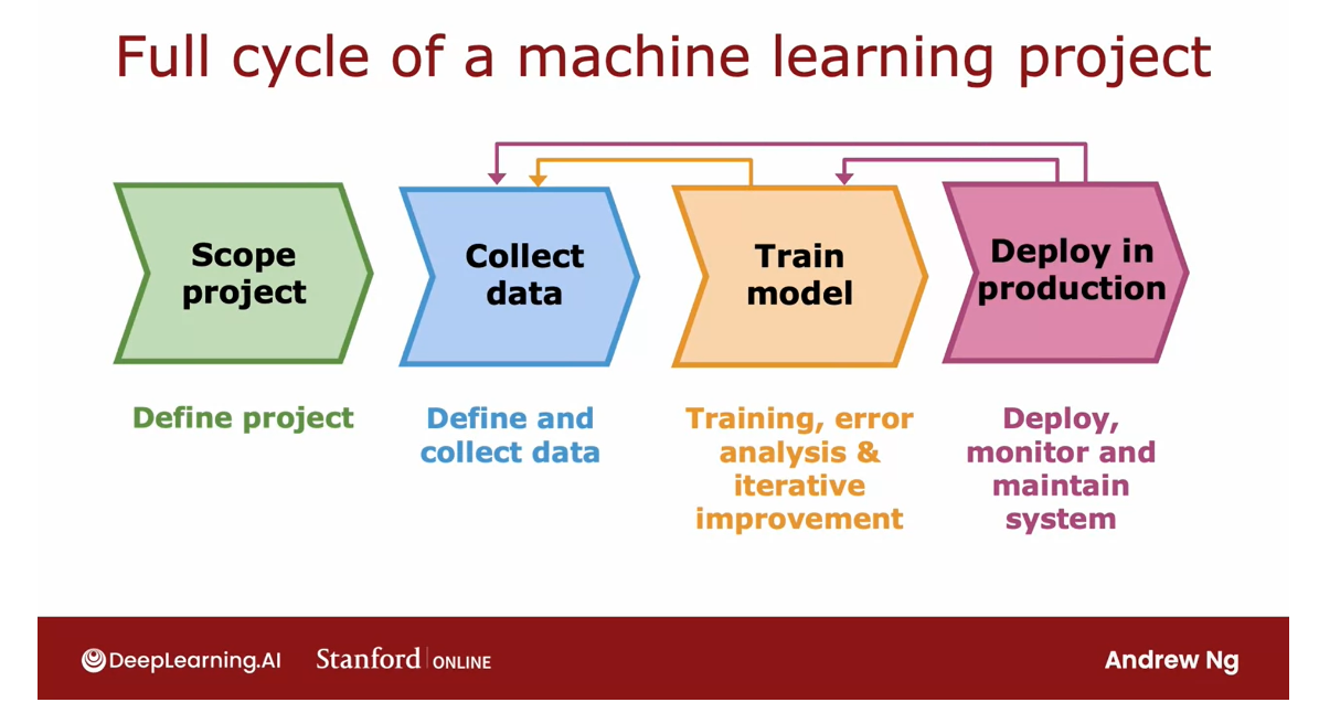
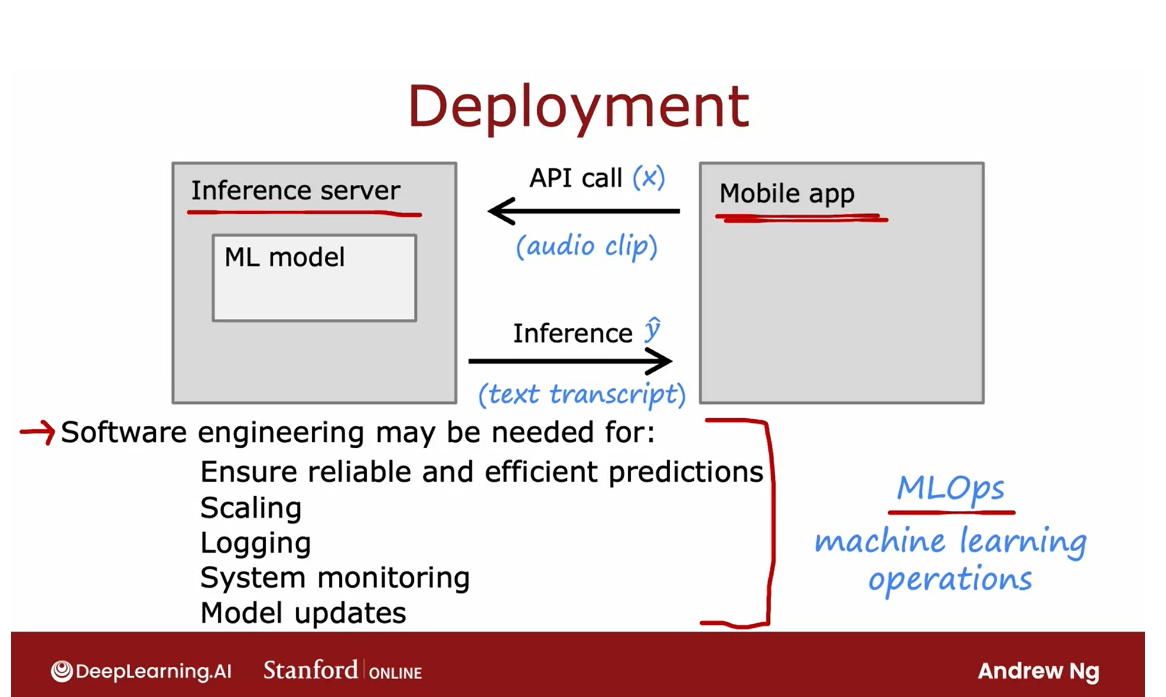
But let me share with you
a little bit more detail about what deploying in
production might look like.

After you’ve trained a high performing
machine learning model, say a speech recognition model, a common way to deploy the
model would be to take your machine learning model
and implement it in a server, which I’m going to call
an inference server, whose job it is to call your
machine learning model, your trained model, in order to make predictions.

Then if your team has
implemented a mobile app, say a social application, then when a user talks
to the mobile app, the mobile app can then
make an API call to pass to your inference server
the audio clip that was recorded and the
inference server’s job is supply the machine
learning model to it and then return to it the
prediction of your model, which in this case would be the text transcripts
of what was said.

This would be a common
way of implementing an application that calls via the API and inference
server that has your model repeatedly
make predictions based on the input, x.

This were common pattern where depend on the application
does implemented.

You have an API call to give your learning
algorithm D input, x, and your machine
learning model within output to prediction, say y hat.

To implement this some
software engineering may be needed to write all the code that does
all of these things.

Depending on whether
your application needs to serve just
a few handful of users or millions of users the amounts of software engineer needed can be quite different.

I’ve build software that serve just a handful of users on
my laptop and I’ve also built software that serves hundreds of millions
of users requiring significant data
center resources.

Depending on scale
application needed, software engineering may
be needed to make sure that your inference
server is able to make reliable and
efficient predictions of the not too higher
computational cost.

Software engineering
may be needed to manage scaling to a large
number of users.

You often want to
log the data you’re getting both the inputs, x, as well as the predictions, y hat, assuming that user privacy and consent
allows you to store this data.

This data, if you
can access to it, is also very useful
for system monitoring.

For example, I once built a
speech recognition system on a certain dataset that
I had but when there were new celebrities
that suddenly became well-known
or elections cause new politicians to become elected and people
will search for these new names that were not in the training set and then
my system did poorly on.

It was because we
were monitoring the system allowed us to figure out when the data was shifting and the algorithm
was becoming less accurate.

This allowed us to retrain the model and then to carry out a model update to replace the
old model with a new one.

Deployment process requires some amounts of software engineering.

The deployment process can require some amounts of
software engineering.

For some applications, if you’re just running it on a laptop or on a
one or two servers, maybe not that much software
engineering is needed.

Depending on the team
you’re working on, it is possible that you built the machine learning
model but there could be a different team responsible
for deploying it.

MLOps: Machine Learning Operations

This refers to the practice of how to systematically build and deploy and maintain machine learning systems.

But there is a growing field in machine learning
called MLOps. This stands for Machine
Learning Operations.

This refers to the
practice of how to systematically build and deploy and maintain machine
learning systems.

To do all of these
things to make sure that your machine learning model
is reliable, scales well, has good laws, is monitored, and then you have the
opportunity to make updates to the model as appropriate
to keep it running well.

For example, if
you are deploying your system to millions
of people you may want to make sure you have a highly optimized
implementations so that the compute cost of serving millions of people
is not too expensive.

In this and the last
parsers I spent a lot of time talking
about how to train a machine learning model and got this absolutely the
critical piece to making sure you have a
high performance system.

If you ever have to deploy
system to millions of people, these are some additional steps that you probably
have to address. Think about the [inaudible]
at that point as well.

Before moving on
from the topic of the machine learning
development process, there’s one more set of ideas that I want
to share with you that relates to the ethics of building machine
learning systems. This is a crucial topic for many applications so let’s take a look at this
in the next video.

Fairness, bias, and ethics

Reasonably fair, reasonably free from bias

Machine learning algorithms today
are affecting billions of people. You’ve heard me mention ethics
in other videos before.

And I hope that if you’re building
a machine learning system that affects people that you give some thought
to making sure that your system is reasonably fair,
reasonably free from bias.

And that you’re taking a ethical
approach to your application.

Let’s take a look at some issues
related to fairness, bias and ethics.

Unfortunately in the history of machine
learning that happened a few systems, some widely publicized, that turned out to exhibit a completely
unacceptable level of bias.

For example, there was a hiring two that was once
shown to discriminate against women.

The company that built
the system stopped using it, but one wishes that the system had never
been rolled out in the first place.

Or there was also well documented
example of face recognition systems that match dark skinned individuals to
criminal mug shots much more often than lighter skinned individuals.

And clearly this is not acceptable and
we should Yeah, that’s where the community at just not building and deploying
systems with a problem like this.

In the first place, there happens
systems that gave bank loan approvals in a way that was biased and
discriminated against subgroups.

And we also really like learning
algorithms to not have the toxic effect of reinforcing negative stereotypes.

For example, I have a daughter and
if she searches online for certain professions and doesn’t see anyone
that looks like her, I would hate for that to discourage her from
taking on certain professions.

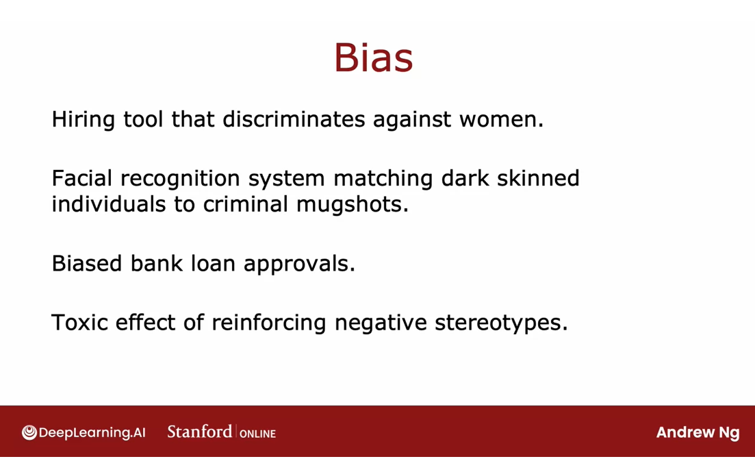
Adverse use cases, negative use cases

In addition to the issues of bias and
fair treatment of individuals, there have also been adverse use cases or negative use cases of
machine learning algorithms.

For example,
there was this widely cited and widely viewed video release with full
disclosure and full transparency.

By the company buzzfeed of a deepfake
of former US President Barack Obama and you can actually find and
watch the whole video online if you want.

But the company that
created this video did so full transparency and full disclosure.

But clearly using this technology to
generate fake videos without consent and without disclosure would be unethical.

We’ve also seen unfortunately social
media sometimes spreading toxic or incendiary speech because optimizing for user engagement has led
to algorithms doing so.

There have been boats that were
used to generate fake content for either commercial purposes such as
posting fake comments on products or for political purposes.

And there are users of machine
learning to build harmful products, commit fraud and so on. And in parts of the machine
learning world, just as an email, there has been a battle between
the spammers and the anti spam community.

I am seeing today in for
example, the financial industry, a battle between people trying to commit
fraud and the people fighting fraud.

And unfortunately machine learning is
used by some of the fraudsters and some of the standards.

So for goodness sakes please don’t
build a machine learning system that has a negative impact on society. And if you are asked to work on an
application that you consider unethical, I urge you to walk away for
what it’s worth.

There have been multiple times that I have
looked at the project that seemed to be financially sound. You’ll make money for some company.

But I have killed the project just on
ethical grounds because I think that even though the financial case will sound, I
felt that it makes the world worse off and I just don’t ever want to be
involved in a project like that.

Ethics is a very complicated and very rich
subject that humanity has studied for at least a few 1000 years.

When aI became more widespread, I actually
went and read up multiple books on philosophy and multiple books on ethics
because I was hoping naively it turned out to come up with if only there’s
a checklist of five things we could do and so as we do these five things then
we can be ethical, but I failed And I don’t think anyone has ever managed
to come up with a simple checklist of things to do to give that level of
concrete guidance about how to be ethical.

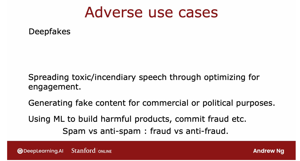
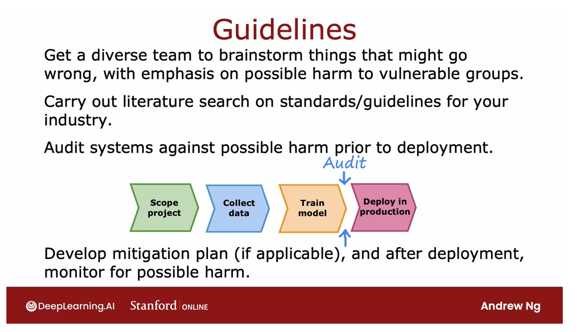
So what I hope to share with you instead
is not a checklist because I wasn’t even come up with one with just some
general guidance and some suggestions for how to make sure the work is less
bias more fair and more ethical.

And I hope that some of these guidance, some which would be relatively general
will help you with your work as well.

So here are some suggestions for
making your work more fair, less biased and more ethical when before
deploying a system that could create harm.

diversity on multiple dimensions ranging from gender to ethnicity to culture, to many other traits.

I will usually try to assemble
a diverse team to brainstorm possible things that might go wrong with
an emphasis on possible harm.

Two vulnerable groups I found many
times in my life that having a more diverse team and by diverse I mean,
diversity on multiple dimensions ranging from gender to ethnicity
to culture, to many other traits.

I found that having more diverse teams
actually causes a team collectively to be better at coming up with ideas
about things that might go wrong and it increases the odds that will
recognize the problem and fix it before rolling out the system and having that
cause harm to some particular group.

In addition to having a diversity and
carried out brain storming.

I have also found it useful to carry out
a literature search on any standards or guidelines for your industry or
particular application area, for example, in the financial industry, there are
starting to be established standards for what it means to be a system.

So they want that decides who to
approve those two, what it means for a system like that to be reasonably
fair and free from bias and those standards that still
emerging in different sectors could inform your work
depending on what you’re working on.

Audit the system against this identified dimensions

After identifying possible problems. I found it useful to then
audit the system against this identified dimensions
of possible home.

Prior to deployment,
you saw in the last video, the full cycle of machine
learning project.

And one key step that’s often a crucial
line of defense against deploying something problematic is after
you’ve trained the model.

But before you deployed in production, if
the team has brainstormed, then it may be biased against certain subgroups such as
certain genders or certain ethnicities.

You can then order the system to measure
the performance to see if it really is bias against certain genders or
ethnicities or other subgroups and to make sure that any problems
are identified and fixed. Prior to deployment.

Mitigation plan

Finally, I found it useful to develop
a mitigation plan if applicable.

And one simple mitigation plan would
be to roll back to the earlier system that we knew was reasonably fair.

And then even after deployment
to continue to monitor harm so that you can then trigger
a mitigation plan and act quickly in case there is
a problem that needs to be addressed.

For example, all of the self driving car
teams prior to rolling out self driving cars on the road had developed
mitigation plans for what to do in case the car ever
gets involved in an accident so that if the car was ever in an accident,
there was already a mitigation plan that they could execute immediately rather
than have a car got into an accident and then only scramble after the fact
to figure out what to do.

I’ve worked on many machine learning
systems and let me tell you the issues of ethics, fairness and
bias issues we should take seriously.

It’s not something to brush off. It’s not something to take likely.

Now of course, there’s some projects with more serious
ethical implications than others.

For example, if I’m building a neural
network to decide how long to roast my coffee beans, clearly,
the ethical implications of that seems significantly less than if, say you’re
building a system to decide what loans. Bank loans are approved, which if it’s
buyers can cause significant harm.

But I hope that all of
us collectively working in machine learning can keep on
getting better debate these issues.

Spot problems, fix them before they cause
harm so that we collectively can avoid some of the mistakes that the machine
learning world had made before because this stuff matters and the systems
we built can affect a lot of people.

And so that’s it on the process of
developing a machine learning system and congratulations on getting to the end
of this week’s required videos.

I have just two more optional
videos this week for you on addressing skewed data sets and
that means steve says where the ratio of positive To negative
examples is very far from 50, 50.

And it turns out that some special
techniques are needed to address machine learning applications like that. So I hope to see you in the next
video optional video on how to handle skewed data sets.

[6] Practice quiz: Machine learning development process

Practice quiz: Machine learning development process

Latest Submission Grade 100%

Question 1

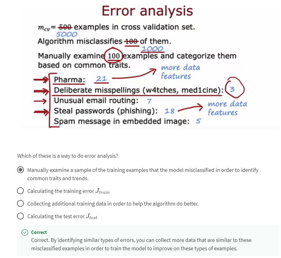
Correct. By identifying similar types of errors, you can collect more data that are similar to these misclassified examples in order to train the model to improve on these types of examples.

Modifying existing data (such as images, or audio) is called data augmentation.

Question 3

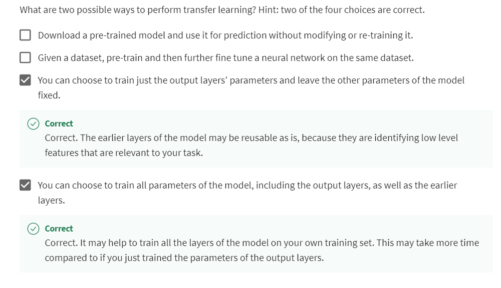
[7] Skewed datasets (optional)

Error metrics for skewed datasets

If the ratio of positive to negative examples is very skewed, then it turns out that the usual error metrics like accuracy don’t work well.

If you’re working on a
machine learning application where the ratio of positive to negative examples
is very skewed, very far from 50-50, then it turns out that the usual error metrics like accuracy don’t work that well.

Let’s start with an example.

Let’s say you’re training a binary classifier to
detect a rare disease in patients based on lab tests or based on other data
from the patients.

Y is equal to 1
if the disease is present and y is
equal to 0 otherwise.

Suppose you find that you’ve achieved one percent
error on the test set, so you have a 99 percent
correct diagnosis.

This seems like a great outcome.

Rare disease

But it turns out that if
this is a rare disease, so y is equal to 1, very rarely, then this may not be as
impressive as it sounds.

Specifically, if it is a
rare disease and if only 0.5 percent of the patients in your population
have the disease, then if instead you
wrote the program, that just said,
print y equals 0. It predicts y equals
0 all the time.

This very simple even
non-learning algorithm, because it just says y
equals 0 all the time, this will actually
have 99.5 percent accuracy or 0.5 percent error.

This really dumb algorithm outperforms your
learning algorithm which had one percent error, much worse than
0.5 percent error.

But I think a piece of software that just
prints y equals 0, is not a very useful
diagnostic tool.

What this really means
is that you can’t tell if getting one percent error is actually a good result
or a bad result.

In particular, if you have one algorithm that achieves
99.5 percent accuracy, different one that achieves
99.2 percent accuracy, different one that achieves
99.6 percent accuracy.

It’s difficult to know which of these is actually
the best algorithm.

Because if you have an algorithm that achieve 0.5
percent error and a different one that achieves
one percent error and a different one that
achieves 1.2 percent error, it’s difficult to know which of these is
the best algorithm.

Because the one with
the lowest error may be is not particularly
useful prediction like this that always
predicts y equals 0 and never ever diagnose any patient
as having this disease.

Quite possibly an algorithm
that has one percent error, but that at least diagnosis
some patients as having the disease could be
more useful than just printing y equals
0 all the time.

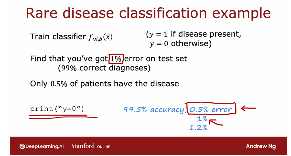
With skewed data sets: use different error metrics, a common pair of error metrics: precision and recall

When working on problems
with skewed data sets, we usually use a different
error metric rather than just classification error to figure out how well your learning
algorithm is doing.

In particular, a common pair of error metrics are
precision and recall, which we’ll define on the slide.

In this example, y equals
one will be the rare class, such as the rare disease
that we may want to detect.

Confusion matrix

In particular, to evaluate a learning algorithm’s
performance with one rare class of useful to construct what’s called
a confusion matrix, which is a two-by-two matrix or a two-by-two table
that looks like this.

On the axis on top, I’m going to write
the actual class, which could be one or zero.

On the vertical axis, I’m going to write
the predicted class, which is what did your
learning algorithm predicts on a given example, one or zero?

To evaluate your
algorithm’s performance on the cross-validation set
or the test set say, we will then count up
how many examples? Was the actual class, 1, and the predicted class 1?

Maybe you have 100
cross-validation examples and on 15 of them, the learning algorithm
had predicted one and the actual
label was also one.

Over here you would
count up the number of examples in C or
cross-validation set where the actual class was zero and your
algorithm predicted one.

Maybe you’ve five
examples there and here predicted Class
0, actual Class 1.

You have 10 examples
and let’s say 70 examples with predicted
Class 0 and actual Class 0.

In this example, the skew isn’t as extreme as what I had
on the previous slide.

Because in these 100 examples in your cross-validation set, we have a total of 25 examples where the
actual class was one and 75 where the
actual class was zero by adding up these
numbers vertically.

You’ll notice also that I’m
using different colors to indicate these four
cells in the table.

I’m actually going to give
names to these four cells.

True positive

When the actual class is one and the predicted
class is one, we’re going to call
that a true positive because you predicted positive and it was true there’s
a positive example.

True negative

In this cell on the lower right, where the actual class is zero and the predicted
class is zero, we will call that
a true negative because you predicted
negative and it was true.

It really was a
negative example.

False positive

This cell on the upper
right is called a false positive
because the algorithm predicted positive,
but it was false.

It’s not actually positive, so this is called
a false positive.

False negative

This cell is called
the number of false negatives
because the algorithm predicted zero,
but it was false.

It wasn’t actually negative. The actual class was one.

Precision

对于我们预测为病人的情况来说，真正得病的占比多少？

$Precision=\frac{Truepositives}{PredictedPositive}$

Recall

对于真正得病的人来说，我们预测他们得病的占比是多少？

$Recall=\frac{Truepositives}{ActualPositive}$

Divide the classifications into four cells

Having divided the
classifications into these four cells, two common metrics
you might compute are then the precision and recall.

Precision: of all the examples you predicted as positive, what fraction did we actually get right.

Here’s what they mean.

The precision of the
learning algorithm computes of all the patients where we
predicted y is equal to 1, what fraction actually
has the rare disease.

In other words, precision
is defined as the number of true positives divided by the number classified
as positive.

In other words, of
all the examples you predicted as positive, what fraction did we
actually get right.

Another way to write
this formula would be true positives divided
by true positives plus false positives
because it is by summing this cell and this cell that you end up with
the total number that was predicted as positive.

In this example, the
numerator, true positives, would be 15 and
divided by 15 plus 5, and so that’s 15 over 20
or three-quarters, 0.75.

So we say that this
algorithm has a precision of 75 percent because of all the things it
predicted as positive, of all the patients that it thought has this rare disease, it was right 75
percent of the time.

Recall: of all the patients that actually have the rare disease, what fraction did we correctly detect as having it

The second metric that is
useful to compute is recall.

Recall ask, of all the patients that actually
have the rare disease, what fraction did we correctly
detect as having it?

Recall is defined as the number
of true positives divided by the number of
actual positives.

Alternatively, we can
write that as number of true positives divided by the
number of actual positives.

Well, it’s this cell
plus this cell. So it’s actually the number
of true positives plus the number of false
negatives because it’s by summing up
this upper-left cell and this lower-left cell that you get the number of
actual positive examples.

In our example, this would
be 15 divided by 15 plus 10, which is 15 over 25, which is 0.6 or 60 percent.

This learning
algorithm would have 0.75 precision and 0.60 recall.

You notice that this
will help you detect if the learning algorithm is just printing y equals
0 all the time. Because if it predicts
zero all the time, then the numerator of both of these quantities
would be zero.

It has no true positives.

The recall metric in particular helps you detect if the learning algorithm is predicting zero all the time.

The recall metric in
particular helps you detect if the learning algorithm is
predicting zero all the time.

Because if your
learning algorithm just prints y equals 0, then the number of true positives will be zero because it never
predicts positive, and so the recall
will be equal to zero divided by the number
of actual positives, which is equal to zero.

if an algorithm actually predicts zero all the time, precision actually becomes undefined because it’s actually zero over zero.

In general, a learning
algorithm with either zero precision or zero recall is not
a useful algorithm.

But just as a side note, if an algorithm actually
predicts zero all the time, precision actually
becomes undefined because it’s actually zero over. zero.

But in practice, if an algorithm doesn’t predict
even a single positive, we just say that precision
is also equal to zero.

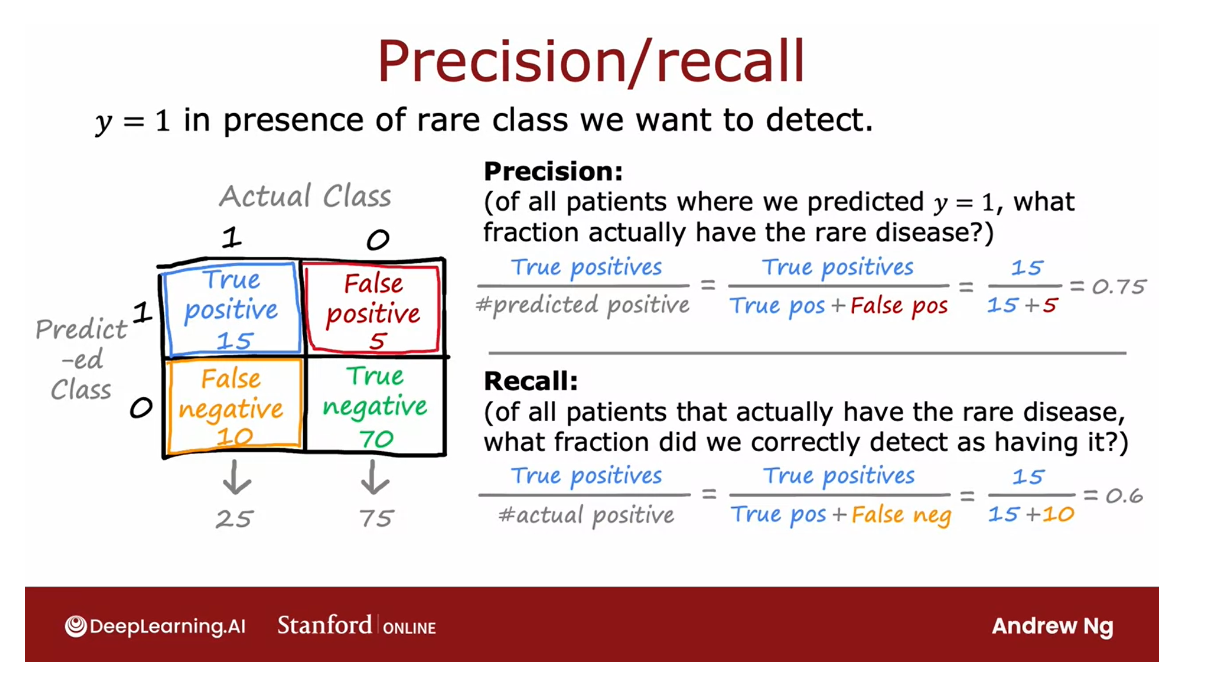
But we’ll find that computing both precision and recall makes it easier to spot if an algorithm is both
reasonably accurate, in that, when it says a
patient has a disease, there’s a good chance the
patient has a disease, such as 0.75 chance
in this example, and also making sure that of all the patients
that have the disease, it’s helping to diagnose a
reasonable fraction of them, such as here it’s finding
60 percent of them.

When you have a rare class, looking at precision and
recall and making sure that both numbers are decently high, that hopefully helps
reassure you that your learning algorithm
is actually useful.

“recall” 一词的动机是这样一个观察结果，即如果你有一组患者或一群患者，那么 recall 衡量的是，在所有患有该疾病的患者中，有多少人被准确诊断为患有该疾病。

The term recall was motivated
by this observation that if you have a group of patients or
population of patients, then recall measures, of all the patients
that have the disease, how many would you have accurately diagnosed
as having it.

So when you have skewed classes or a rare class that
you want to detect, precision and recall
helps you tell if your learning
algorithm is making good predictions or
useful predictions.

Now that we have
these metrics for telling how well your
learning algorithm is doing, in the next video, let’s take a look at how to
trade-off between precision and recall to try to optimize the performance of your
learning algorithm.

Trading off precision and recall

In the ideal case, we like for learning
algorithms that have high precision and high recall.

高精度意味着，如果对患者的诊断有这种罕见的疾病，很可能患者确实有这种疾病，这是一个准确的诊断。

High precision
would mean that if a diagnosis of patients
have that rare disease, probably the patient does have it and it’s an
accurate diagnosis.

高recall意味着如果有一个患者患有这种罕见的疾病，算法可能会正确地识别出他们确实患有这种疾病。

High recall means that if there’s a patient with
that rare disease, probably the algorithm
will correctly identify that they do
have that disease.

But it turns out that in
practice there’s often a trade-off between
precision and recall.

In this video, we’ll take
a look at that trade-off and how you can pick a good
point along that trade-off.

Here are the definitions from the last video on precision and recall, I’ll just
write them here.

Well, precision is the number of true positives divided by the total number
that was predicted positive, and recall is the number of
true positives divided by the total actual
number of positives.

If you’re using logistic
regression to make predictions, then the logistic
regression model will output numbers
between 0 and 1.

We would typically
threshold the output of logistic
regression at 0.5 and predict 1 if f of x is
greater than equal to 0.5 and predict 0 if
it’s less than 0.5.

But suppose we want to
predict that y is equal to 1. That is, the rare disease is present only if we’re
very confident.

如果我们的理念是，无论何时我们预测患者患有疾病，我们都可能不得不送他们接受可能的大量和昂贵的治疗。
如果疾病的后果没有那么严重，即使不积极治疗，那么只有在我们非常自信的情况下，我们才能预测y等于1。

If our philosophy is, whenever we predict that
the patient has a disease, we may have to send them for possibly invasive and
expensive treatment.

If the consequences of the
disease aren’t that bad, even if left not
treated aggressively, then we may want to
predict y equals 1 only if we’re very confident.

In that case, we
may choose to set a higher threshold where we will predict y is 1 only if f of x is greater than or equal to 0.7, so this is saying we’ll
predict y equals 1 only we’re at least
70 percent sure, rather than just 50
percent sure and so this number also becomes 0.7.

Notice that these
two numbers have to be the same because
it’s just depending on whether it’s greater
than or equal to or less than this number
that you predict 1 or 0.

By raising this threshold, you predict y equals 1 only if you’re pretty confident
and what that means is that precision will increase because whenever
you predict one, you’re more likely
to be right so raising the thresholds will
result in higher precision, but it also results in lower recall because
we’re now predicting one less often and so of the total number of
patients with the disease, we’re going to correctly
diagnose fewer of them.

By raising this
threshold to 0.7, you end up with higher
precision, but lower recall.

In fact, if you
want to predict y equals 1 only if you
are very confident, you can even raise this higher
to 0.9 and that results in an even higher precision and so whenever you predict
the patient has the disease, you’re probably right and this will give you a very
high precision.

The recall will go
even further down.

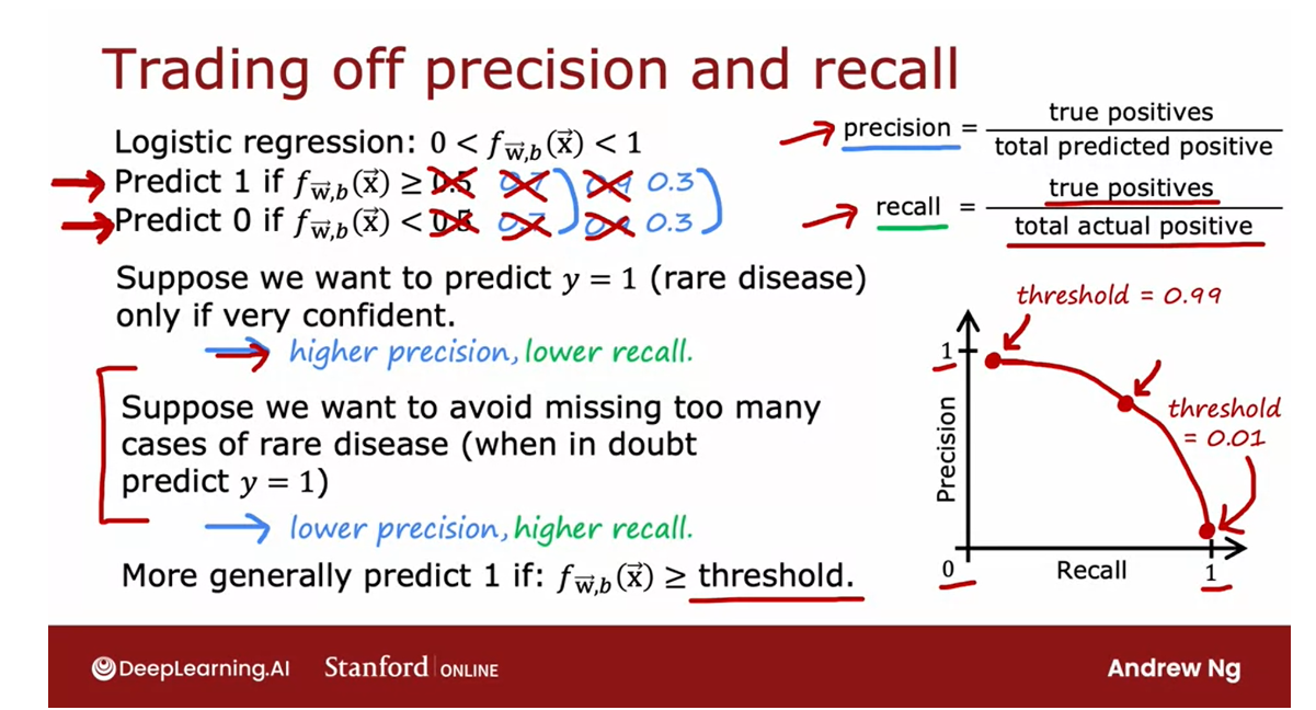
On the flip side, suppose we want to avoid missing too many cases of
the rare disease, so if what we want
is when in doubt, predict y equals 1, this might be the case where if treatment is not
too invasive or painful or expensive but leaving a disease untreated has much worse consequences
for the patient.

In that case, you might say, when in doubt in
the interests of safety let’s just
predict that they have it and consider
them for treatment because untreated cases
could be quite bad.

If for your application, that is the better way
to make decisions, then you would take this
threshold instead lower it, say, set it to 0.3.

In that case, you
predict one so long as you think there’s maybe
a 30 percent chance or better of the disease
being present and you predict zero only
if you’re pretty sure that the disease is absent.

As you can imagine, the impact on precision
and recall will be opposite to what
you saw up here, and lowering this
threshold will result in lower precision because
we’re now looser, we’re more willing to predict
one even if we aren’t sure but to result in higher recall, because of all the patients
that do have that disease, we’re probably going to
correctly identify more of them.

More generally, we have
the flexibility to predict one only if f is above some threshold and by
choosing this threshold, we can make different trade-offs between precision and recall.

It turns out that for
most learning algorithms, there is a trade-off between
precision and recall. Precision and recall
both go between zero and one and if you were to set
a very high threshold, say a threshold of 0.99, then you enter with
very high precision, but lower recall and as you reduce the value
of this threshold, you then end up
with a curve that trades off precision and
recall until eventually, if you have a very
low threshold, so the threshold equals 0.01, then you end up with very low precision but
relatively high recall.

Sometimes by
plotting this curve, you can then try to
pick a threshold which corresponds to picking
a point on this curve.

The balances, the cost of false positives and false
negatives or the balances, the benefits of high
precision and high recall.

Plotting precision and recall
for different values of the threshold allows you to
pick a point that you want.

Notice that picking the
threshold is not something you can really do with cross-validation because it’s up to you to specify
the best points.

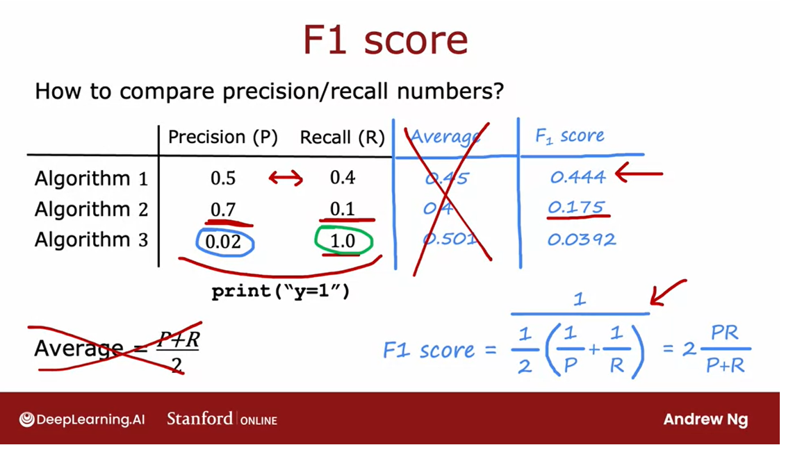
For many applications, manually picking the threshold to trade-off precision and recall will be what you end up doing.

For many applications, manually
picking the threshold to trade-off precision and recall will be what you end up doing.

there is another metric called the F1 score that is sometimes used to automatically combine precision recall to help you pick the best value or the best trade-off between the two.

It turns out that if you
want to automatically trade-off precision and recall rather than have
to do so yourself, there is another metric called the F1 score that is
sometimes used to automatically combine
precision recall to help you pick the best value or the best trade-off
between the two.

One challenge with precision
recall is you’re now evaluating your algorithms
using two different metrics, so if you’ve trained three different algorithms and the precision-recall
numbers look like this, is not that obvious how to
pick which algorithm to use.

If there was an algorithm that’s better on precision
and better on recall, then you probably want
to go with that one.

But in this example, Algorithm 2 has the
highest precision, but Algorithm 3 has
the highest recall, and Algorithm 1 trades
off the two in-between, and so no one algorithm is
obviously the best choice.

In order to help you decide
which algorithm to pick, it may be useful
to find a way to combine precision and
recall into a single score, so you can just look
at which algorithm has the highest score and
maybe go with that one.

One way you could
combine precision and recall is to take the average, this turns out not
to be a good way, so I don’t really
recommend this.

But if we were to
take the average, you get 0.45, 0.4, and 0.5. But it turns out that computing the average and
picking the algorithm with the highest average between precision and
recall doesn’t work that well because this algorithm
has very low precision, and in fact, this corresponds maybe to an algorithm
that actually does print y equals 1 and diagnosis all patients
as having the disease, that’s why recall is perfect but the
precision is really low.

Algorithm 3 is actually not a particularly useful algorithm, even though the average
between precision and recall is quite high.

Let’s not use the average
between precision and recall.

the F1 score is a way of combining P and R （precision and recall） but that gives more emphasis to whichever of these values is lower.

Instead, the most
common way of combining precision recall is a compute something called the F1 score, and the F1 score is a way of combining P and R precision and recall but that gives more emphasis to whichever
of these values is lower.

Because it turns out
if an algorithm has very low precision or very low recall is
pretty not that useful.

The F1 score is a way
of computing an average of sorts that pays more
attention to whichever is lower.

The formula for computing
F1 score is this, you’re going to compute
one over P and one over R, and average them, and then take the
inverse of that.

Rather than averaging P
and R precision recall we’re going to average one
over P and one over R, and then take one over that. If you simplify this
equation it can also be computed as follows.

But by averaging one over P
and one over R this gives a much greater emphasis
to if either P or R turns out to be very small.

If you were to compute the F1 score for these
three algorithms, you’ll find that the F1 score
for Algorithm 1 is 0.444, and for the second
algorithm is 0.175. You notice that 0.175 is much closer to the
lower value than the higher value and for the
third algorithm is 0.0392.

F1 score gives a way to trade-off precision and
recall, and in this case, it will tell us that maybe the first algorithm is better than the second
or the third algorithms.

F1 score: harmonic mean of P and R

By the way, in math, this equation is also called the harmonic mean of P and R, and the harmonic mean
is a way of taking an average that emphasizes
the smaller values more.

But for the purposes
of this class, you don’t need to worry about that terminology of
the harmonic mean.

Congratulations on getting to the last video of this
week and thank you also for sticking
with me through these two optional videos.

In this week, you’ve learned
a lot of practical tips, practical advice for how to build a machine learning system, and by applying these ideas, I think you’d be
very effective at building machine
learning algorithms.

Next week, we’ll come
back to talk about another very powerful
machine learning algorithm.

In fact, of the advanced
techniques that why we use in many commercial
production settings, I think at the top
of the list would be neural networks and
decision trees.

Next week we’ll talk
about decision trees, which I think will be another very powerful technique that you’re going to use to build many successful
applications as well. I look forward to
seeing you next week.

[8] Practice Lab: Advice for applying machine learning

Grade

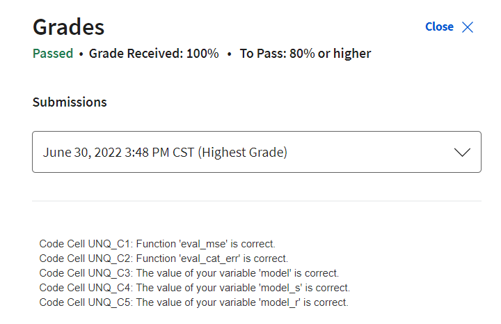
Practice Lab - Advice for Applying Machine Learning

In this lab, you will explore techniques to evaluate and improve your machine learning models.

1 - Packages

First, let’s run the cell below to import all the packages that you will need during this assignment.

• numpy is the fundamental package for scientific computing Python.
• matplotlib is a popular library to plot graphs in Python.
• scikitlearn is a basic library for data mining
• tensorflow a popular platform for machine learning.

import numpy as np
%matplotlib widget
import matplotlib.pyplot as plt
from sklearn.linear_model import LinearRegression, Ridge
from sklearn.preprocessing import StandardScaler, PolynomialFeatures
from sklearn.model_selection import train_test_split
from sklearn.metrics import mean_squared_error
import tensorflow as tf
from tensorflow.keras.models import Sequential
from tensorflow.keras.layers import Dense
from tensorflow.keras.activations import relu,linear
from tensorflow.keras.losses import SparseCategoricalCrossentropy
from tensorflow.keras.optimizers import Adam

import logging
logging.getLogger("tensorflow").setLevel(logging.ERROR)

from public_tests_a1 import * 

tf.keras.backend.set_floatx('float64')
from assigment_utils import *

tf.autograph.set_verbosity(0)

2 - Evaluating a Learning Algorithm (Polynomial Regression)

Let’s say you have created a machine learning model and you find it fits your training data very well. You’re done? Not quite. The goal of creating the model was to be able to predict values for new examples.

How can you test your model’s performance on new data before deploying it?
The answer has two parts:

• Split your original data set into “Training” and “Test” sets.
  • Use the training data to fit the parameters of the model
  • Use the test data to evaluate the model on new data
• Develop an error function to evaluate your model.

2.1 Splitting your data set

Lectures advised reserving 20-40% of your data set for testing. Let’s use an sklearn function train_test_split to perform the split. Double-check the shapes after running the following cell.

# Generate some data
X,y,x_ideal,y_ideal = gen_data(18, 2, 0.7)
print("X.shape", X.shape, "y.shape", y.shape)

#split the data using sklearn routine 
X_train, X_test, y_train, y_test = train_test_split(X,y,test_size=0.33, random_state=1)
print("X_train.shape", X_train.shape, "y_train.shape", y_train.shape)
print("X_test.shape", X_test.shape, "y_test.shape", y_test.shape)

Output

X.shape (18,) y.shape (18,)
X_train.shape (12,) y_train.shape (12,)
X_test.shape (6,) y_test.shape (6,)

2.1.1 Plot Train, Test sets

You can see below the data points that will be part of training (in red) are intermixed with those that the model is not trained on (test). This particular data set is a quadratic function with noise added. The “ideal” curve is shown for reference.

fig, ax = plt.subplots(1,1,figsize=(4,4))
ax.plot(x_ideal, y_ideal, "--", color = "orangered", label="y_ideal", lw=1)
ax.set_title("Training, Test",fontsize = 14)
ax.set_xlabel("x")
ax.set_ylabel("y")

ax.scatter(X_train, y_train, color = "red",           label="train")
ax.scatter(X_test, y_test,   color = dlc["dlblue"],   label="test")
ax.legend(loc='upper left')
plt.show()

Output

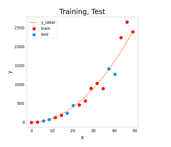
2.2 Error calculation for model evaluation, linear regression

When evaluating a linear regression model, you average the squared error difference of the predicted values and the target values.

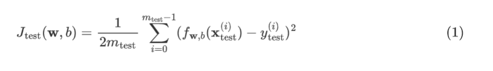
Latex公式

J_\text{test}(\mathbf{w},b) = 
            \frac{1}{2m_\text{test}}\sum_{i=0}^{m_\text{test}-1} ( f_{\mathbf{w},b}(\mathbf{x}^{(i)}_\text{test}) - y^{(i)}_\text{test} )^2 \tag{1}

Exercise 1

Below, create a function to evaluate the error on a data set for a linear regression model.

Code

# UNQ_C1
# GRADED CELL: eval_mse
def eval_mse(y, yhat):
    """ 
    Calculate the mean squared error on a data set.
    Args:
      y    : (ndarray  Shape (m,) or (m,1))  target value of each example
      yhat : (ndarray  Shape (m,) or (m,1))  predicted value of each example
    Returns:
      err: (scalar)             
    """
    m = len(y)
    err = 0.0
    for i in range(m):
    ### START CODE HERE ### 
        err = err + (yhat[i] - y[i]) ** 2
        
    err = err / (2 * m)
    
    ### END CODE HERE ### 
    
    return(err)

Test

y_hat = np.array([2.4, 4.2])
y_tmp = np.array([2.3, 4.1])
eval_mse(y_hat, y_tmp)

# BEGIN UNIT TEST
test_eval_mse(eval_mse)   
# END UNIT TEST

Output

All tests passed.

Hints

def eval_mse(y, yhat):
    """ 
    Calculate the mean squared error on a data set.
    Args:
      y    : (ndarray  Shape (m,) or (m,1))  target value of each example
      yhat : (ndarray  Shape (m,) or (m,1))  predicted value of each example
    Returns:
      err: (scalar)             
    """
    m = len(y)
    err = 0.0
    for i in range(m):
        err_i  = ( (yhat[i] - y[i])**2 ) 
        err   += err_i                                                                
    err = err / (2*m)                    
    return(err)

2.3 Compare performance on training and test data

Let’s build a high degree polynomial model to minimize training error. This will use the linear_regression functions from sklearn. The code is in the imported utility file if you would like to see the details. The steps below are:

• create and fit the model. (‘fit’ is another name for training or running gradient descent).
• compute the error on the training data.
• compute the error on the test data.

# create a model in sklearn, train on training data
degree = 10
lmodel = lin_model(degree)
lmodel.fit(X_train, y_train)

# predict on training data, find training error
yhat = lmodel.predict(X_train)
err_train = lmodel.mse(y_train, yhat)

# predict on test data, find error
yhat = lmodel.predict(X_test)
err_test = lmodel.mse(y_test, yhat)

The computed error on the training set is substantially less than that of the test set.

print(f"training err {err_train:0.2f}, test err {err_test:0.2f}")

Output

training err 58.01, test err 171215.01

The following plot shows why this is. The model fits the training data very well. To do so, it has created a complex function. The test data was not part of the training and the model does a poor job of predicting on this data.
This model would be described as 1) is overfitting, 2) has high variance 3) ‘generalizes’ poorly.

# plot predictions over data range 
x = np.linspace(0,int(X.max()),100)  # predict values for plot
y_pred = lmodel.predict(x).reshape(-1,1)

plt_train_test(X_train, y_train, X_test, y_test, x, y_pred, x_ideal, y_ideal, degree)

Output

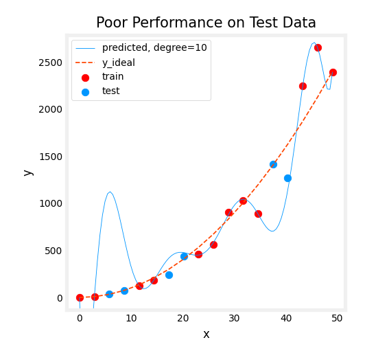
The test set error shows this model will not work well on new data. If you use the test error to guide improvements in the model, then the model will perform well on the test data… but the test data was meant to represent new data.
You need yet another set of data to test new data performance.

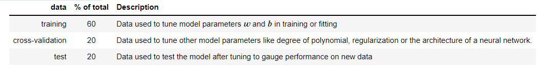
The proposal made during lecture is to separate data into three groups. The distribution of training, cross-validation and test sets shown in the below table is a typical distribution, but can be varied depending on the amount of data available.

data	% of total	Description
training	60	Data used to tune model parameters $w$ and $b$ in training or fitting
cross-validation	20	Data used to tune other model parameters like degree of polynomial, regularization or the architecture of a neural network.
test	20	Data used to test the model after tuning to gauge performance on new data

Let’s generate three data sets below. We’ll once again use train_test_split from sklearn but will call it twice to get three splits:

# Generate  data
X,y, x_ideal,y_ideal = gen_data(40, 5, 0.7)
print("X.shape", X.shape, "y.shape", y.shape)

#split the data using sklearn routine 
X_train, X_, y_train, y_ = train_test_split(X,y,test_size=0.40, random_state=1)
X_cv, X_test, y_cv, y_test = train_test_split(X_,y_,test_size=0.50, random_state=1)
print("X_train.shape", X_train.shape, "y_train.shape", y_train.shape)
print("X_cv.shape", X_cv.shape, "y_cv.shape", y_cv.shape)
print("X_test.shape", X_test.shape, "y_test.shape", y_test.shape)

Output

X.shape (40,) y.shape (40,)
X_train.shape (24,) y_train.shape (24,)
X_cv.shape (8,) y_cv.shape (8,)
X_test.shape (8,) y_test.shape (8,)

3 - Bias and Variance

Above, it was clear the degree of the polynomial model was too high. How can you choose a good value? It turns out, as shown in the diagram, the training and cross-validation performance can provide guidance. By trying a range of degree values, the training and cross-validation performance can be evaluated. As the degree becomes too large, the cross-validation performance will start to degrade relative to the training performance. Let’s try this on our example.

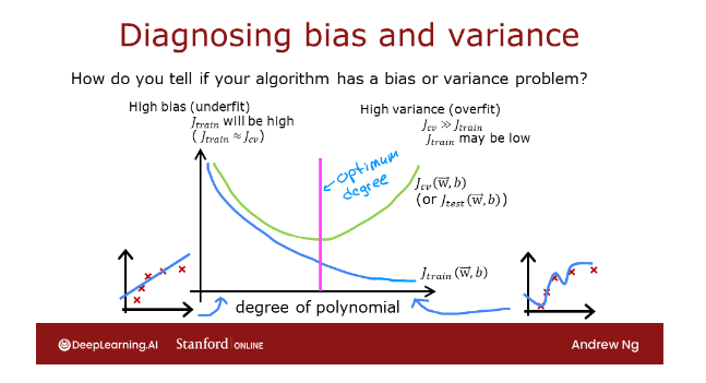
3.1 Plot Train, Cross-Validation, Test

You can see below the datapoints that will be part of training (in red) are intermixed with those that the model is not trained on (test and cv).

fig, ax = plt.subplots(1,1,figsize=(4,4))
ax.plot(x_ideal, y_ideal, "--", color = "orangered", label="y_ideal", lw=1)
ax.set_title("Training, CV, Test",fontsize = 14)
ax.set_xlabel("x")
ax.set_ylabel("y")

ax.scatter(X_train, y_train, color = "red",           label="train")
ax.scatter(X_cv, y_cv,       color = dlc["dlorange"], label="cv")
ax.scatter(X_test, y_test,   color = dlc["dlblue"],   label="test")
ax.legend(loc='upper left')
plt.show()

Output

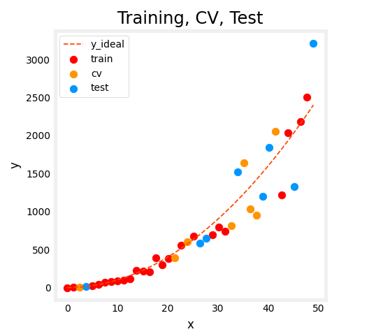
3.2 Finding the optimal degree

In previous labs, you found that you could create a model capable of fitting complex curves by utilizing a polynomial (See Course1, Week2 Feature Engineering and Polynomial Regression Lab). Further, you demonstrated that by increasing the degree of the polynomial, you could create overfitting. (See Course 1, Week3, Over-Fitting Lab). Let’s use that knowledge here to test our ability to tell the difference between over-fitting and under-fitting.

Let’s train the model repeatedly, increasing the degree of the polynomial each iteration. Here, we’re going to use the scikit-learn linear regression model for speed and simplicity.

max_degree = 9
err_train = np.zeros(max_degree)    
err_cv = np.zeros(max_degree)      
x = np.linspace(0,int(X.max()),100)  
y_pred = np.zeros((100,max_degree))  #columns are lines to plot

for degree in range(max_degree):
    lmodel = lin_model(degree+1)
    lmodel.fit(X_train, y_train)
    yhat = lmodel.predict(X_train)
    err_train[degree] = lmodel.mse(y_train, yhat)
    yhat = lmodel.predict(X_cv)
    err_cv[degree] = lmodel.mse(y_cv, yhat)
    y_pred[:,degree] = lmodel.predict(x)
    
optimal_degree = np.argmin(err_cv)+1

Let’s plot the result:

plt.close("all")
plt_optimal_degree(X_train, y_train, X_cv, y_cv, x, y_pred, x_ideal, y_ideal, 
                   err_train, err_cv, optimal_degree, max_degree)

Output

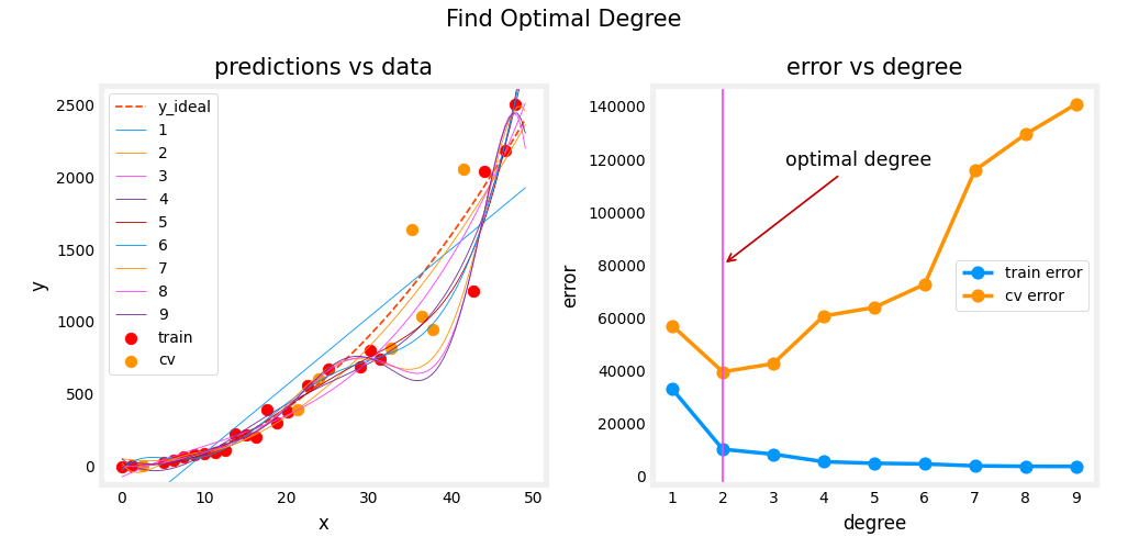
The plot above demonstrates that separating data into two groups, data the model is trained on and data the model has not been trained on, can be used to determine if the model is underfitting or overfitting. In our example, we created a variety of models varying from underfitting to overfitting by increasing the degree of the polynomial used.

• On the left plot, the solid lines represent the predictions from these models. A polynomial model with degree 1 produces a straight line that intersects very few data points, while the maximum degree hews very closely to every data point.
• on the right:
  • the error on the trained data (blue) decreases as the model complexity increases as expected
  • the error of the cross-validation data decreases initially as the model starts to conform to the data, but then increases as the model starts to over-fit on the training data (fails to generalize).

It’s worth noting that the curves in these examples as not as smooth as one might draw for a lecture. It’s clear the specific data points assigned to each group can change your results significantly. The general trend is what is important.

3.3 Tuning Regularization.

In previous labs, you have utilized regularization to reduce overfitting. Similar to degree, one can use the same methodology to tune the regularization parameter lambda ($\lambda$).

Let’s demonstrate this by starting with a high degree polynomial and varying the regularization parameter.

lambda_range = np.array([0.0, 1e-6, 1e-5, 1e-4,1e-3,1e-2, 1e-1,1,10,100])
num_steps = len(lambda_range)
degree = 10
err_train = np.zeros(num_steps)    
err_cv = np.zeros(num_steps)       
x = np.linspace(0,int(X.max()),100) 
y_pred = np.zeros((100,num_steps))  #columns are lines to plot

for i in range(num_steps):
    lambda_= lambda_range[i]
    lmodel = lin_model(degree, regularization=True, lambda_=lambda_)
    lmodel.fit(X_train, y_train)
    yhat = lmodel.predict(X_train)
    err_train[i] = lmodel.mse(y_train, yhat)
    yhat = lmodel.predict(X_cv)
    err_cv[i] = lmodel.mse(y_cv, yhat)
    y_pred[:,i] = lmodel.predict(x)
    
optimal_reg_idx = np.argmin(err_cv) 

Plot

plt.close("all")
plt_tune_regularization(X_train, y_train, X_cv, y_cv, x, y_pred, err_train, err_cv, optimal_reg_idx, lambda_range)

Output

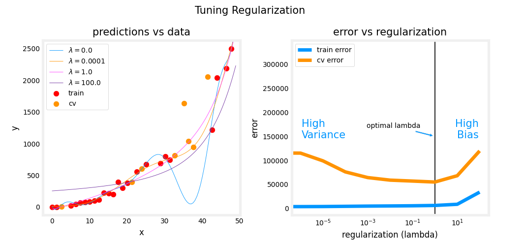
Above, the plots show that as regularization increases, the model moves from a high variance (overfitting) model to a high bias (underfitting) model. The vertical line in the right plot shows the optimal value of lambda. In this example, the polynomial degree was set to 10.

3.4 Getting more data: Increasing Training Set Size (m)

When a model is overfitting (high variance), collecting additional data can improve performance. Let’s try that here.

X_train, y_train, X_cv, y_cv, x, y_pred, err_train, err_cv, m_range,degree = tune_m()
plt_tune_m(X_train, y_train, X_cv, y_cv, x, y_pred, err_train, err_cv, m_range, degree)

Output

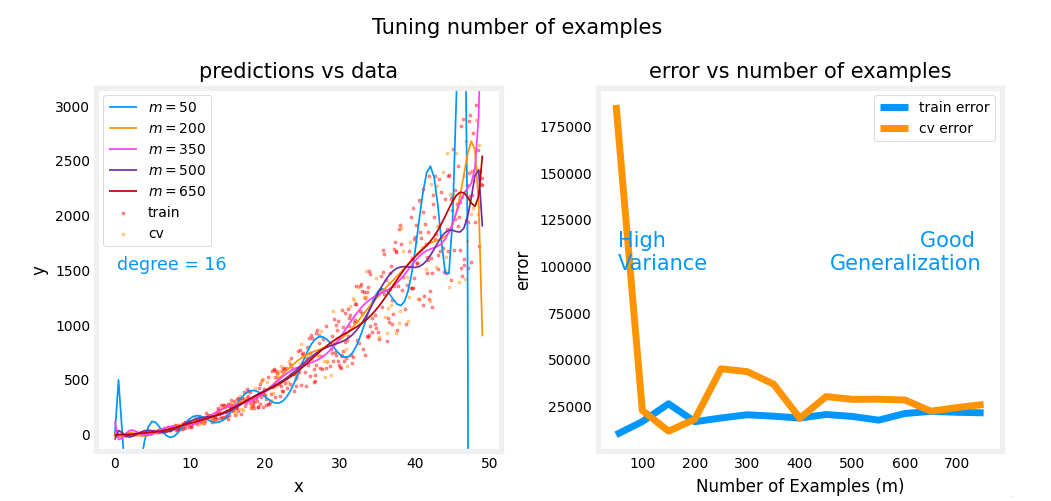
The above plots show that when a model has high variance and is overfitting, adding more examples improves performance. Note the curves on the left plot. The final curve with the highest value of $m$ is a smooth curve that is in the center of the data. On the right, as the number of examples increases, the performance of the training set and cross-validation set converge to similar values. Note that the curves are not as smooth as one might see in a lecture. That is to be expected. The trend remains clear: more data improves generalization.

Note that adding more examples when the model has high bias (underfitting) does not improve performance.

4 - Evaluating a Learning Algorithm (Neural Network)

Above, you tuned aspects of a polynomial regression model. Here, you will work with a neural network model. Let’s start by creating a classification data set.

4.1 Data Set

Run the cell below to generate a data set and split it into training, cross-validation (CV) and test sets. In this example, we’re increasing the percentage of cross-validation data points for emphasis.

# Generate and split data set
X, y, centers, classes, std = gen_blobs()

# split the data. Large CV population for demonstration
X_train, X_, y_train, y_ = train_test_split(X,y,test_size=0.50, random_state=1)
X_cv, X_test, y_cv, y_test = train_test_split(X_,y_,test_size=0.20, random_state=1)
print("X_train.shape:", X_train.shape, "X_cv.shape:", X_cv.shape, "X_test.shape:", X_test.shape)

Output

X_train.shape: (400, 2) X_cv.shape: (320, 2) X_test.shape: (80, 2)

Plot

plt_train_eq_dist(X_train, y_train,classes, X_cv, y_cv, centers, std)

Output

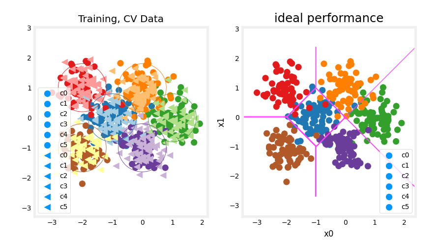
Above, you can see the data on the left. There are six clusters identified by color. Both training points (dots) and cross-validataion points (triangles) are shown. The interesting points are those that fall in ambiguous locations where either cluster might consider them members. What would you expect a neural network model to do? What would be an example of overfitting? underfitting?
On the right is an example of an ‘ideal’ model, or a model one might create knowing the source of the data. The lines represent ‘equal distance’ boundaries where the distance between center points is equal. It’s worth noting that this model would “misclassify” roughly 8% of the total data set.

4.2 Evaluating categorical model by calculating classification error

The evaluation function for categorical models used here is simply the fraction of incorrect predictions:

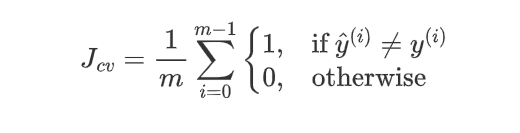
Latex 公式

J_{cv} =\frac{1}{m}\sum_{i=0}^{m-1} 
\begin{cases}
    1, & \text{if $\hat{y}^{(i)} \neq y^{(i)}$}\\
    0, & \text{otherwise}
\end{cases}

Exercise 2

Below, complete the routine to calculate classification error. Note, in this lab, target values are the index of the category and are not one-hot encoded.

# UNQ_C2
# GRADED CELL: eval_cat_err
def eval_cat_err(y, yhat):
    """ 
    Calculate the categorization error
    Args:
      y    : (ndarray  Shape (m,) or (m,1))  target value of each example
      yhat : (ndarray  Shape (m,) or (m,1))  predicted value of each example
    Returns:|
      cerr: (scalar)             
    """
    m = len(y)
    incorrect = 0
    for i in range(m):
    ### START CODE HERE ### 
        if yhat[i] != y[i]:
            incorrect += 1
    cerr = incorrect / m
    ### END CODE HERE ### 
    
    return(cerr)

Test

y_hat = np.array([1, 2, 0])
y_tmp = np.array([1, 2, 3])
print(f"categorization error {np.squeeze(eval_cat_err(y_hat, y_tmp)):0.3f}, expected:0.333" )
y_hat = np.array([[1], [2], [0], [3]])
y_tmp = np.array([[1], [2], [1], [3]])
print(f"categorization error {np.squeeze(eval_cat_err(y_hat, y_tmp)):0.3f}, expected:0.250" )

# BEGIN UNIT TEST  
test_eval_cat_err(eval_cat_err)
# END UNIT TEST
# BEGIN UNIT TEST  
test_eval_cat_err(eval_cat_err)
# END UNIT TEST

Output

categorization error 0.333, expected:0.333
categorization error 0.250, expected:0.250
 All tests passed.
 All tests passed.

Hints

def eval_cat_err(y, yhat):
    """ 
    Calculate the categorization error
    Args:
      y    : (ndarray  Shape (m,) or (m,1))  target value of each example
      yhat : (ndarray  Shape (m,) or (m,1))  predicted value of each example
    Returns:|
      cerr: (scalar)             
    """
    m = len(y)
    incorrect = 0
    for i in range(m):
        if yhat[i] != y[i]:    # @REPLACE
            incorrect += 1     # @REPLACE
    cerr = incorrect/m         # @REPLACE
    return(cerr)  

5 - Model Complexity

Below, you will build two models. A complex model and a simple model. You will evaluate the models to determine if they are likely to overfit or underfit.

5.1 Complex model

Exercise 3

Below, compose a three-layer model:

• Dense layer with 120 units, relu activation
• Dense layer with 40 units, relu activation
• Dense layer with 6 units and a linear activation (not softmax)
  Compile using
• loss with SparseCategoricalCrossentropy, remember to use from_logits=True
• Adam optimizer with learning rate of 0.01.

# UNQ_C3
# GRADED CELL: model
import logging
logging.getLogger("tensorflow").setLevel(logging.ERROR)

tf.random.set_seed(1234)
model = Sequential(
    [
        ### START CODE HERE ### 
        Dense(120, activation="relu"),
        Dense(40, activation="relu"),
        Dense(6, activation="linear")
  
        ### END CODE HERE ### 

    ], name="Complex"
)
model.compile(
    ### START CODE HERE ### 
    loss=SparseCategoricalCrossentropy(from_logits=True),
    optimizer=Adam(0.01),
    ### END CODE HERE ### 
)

Unit Test

# BEGIN UNIT TEST
model.fit(
    X_train, y_train,
    epochs=1000
)
# END UNIT TEST

# BEGIN UNIT TEST
model.summary()

model_test(model, classes, X_train.shape[1]) 
# END UNIT TEST

Output

Model: "Complex"
_________________________________________________________________
 Layer (type)                Output Shape              Param #   
=================================================================
 dense_3 (Dense)             (None, 120)               360       
                                                                 
 dense_4 (Dense)             (None, 40)                4840      
                                                                 
 dense_5 (Dense)             (None, 6)                 246       
                                                                 
=================================================================
Total params: 5,446
Trainable params: 5,446
Non-trainable params: 0
_________________________________________________________________
All tests passed!

Hints

Summary should match this (layer instance names may increment )

Model: "Complex"
_________________________________________________________________
Layer (type)                 Output Shape              Param #   
=================================================================
L1 (Dense)                   (None, 120)               360       
_________________________________________________________________
L2 (Dense)                   (None, 40)                4840      
_________________________________________________________________
L3 (Dense)                   (None, 6)                 246       
=================================================================
Total params: 5,446
Trainable params: 5,446
Non-trainable params: 0
_________________________________________________________________

More hints

tf.random.set_seed(1234)
model = Sequential(
    [
        Dense(120, activation = 'relu', name = "L1"),      
        Dense(40, activation = 'relu', name = "L2"),         
        Dense(classes, activation = 'linear', name = "L3")  
    ], name="Complex"
)
model.compile(
    loss=tf.keras.losses.SparseCategoricalCrossentropy(from_logits=True),          
    optimizer=tf.keras.optimizers.Adam(0.01),   
)

model.fit(
    X_train,y_train,
    epochs=1000
)                        

make a model for plotting routines to call

#make a model for plotting routines to call
model_predict = lambda Xl: np.argmax(tf.nn.softmax(model.predict(Xl)).numpy(),axis=1)
plt_nn(model_predict,X_train,y_train, classes, X_cv, y_cv, suptitle="Complex Model")

Output

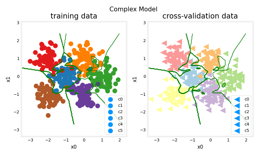
This model has worked very hard to capture outliers of each category. As a result, it has miscategorized some of the cross-validation data. Let’s calculate the classification error.

training_cerr_complex = eval_cat_err(y_train, model_predict(X_train))
cv_cerr_complex = eval_cat_err(y_cv, model_predict(X_cv))
print(f"categorization error, training, complex model: {training_cerr_complex:0.3f}")
print(f"categorization error, cv,       complex model: {cv_cerr_complex:0.3f}")

Output

categorization error, training, complex model: 0.003
categorization error, cv,       complex model: 0.122

5.1 Simple model

Now, let’s try a simple model

Exercise 4

Below, compose a two-layer model:

• Dense layer with 6 units, relu activation
• Dense layer with 6 units and a linear activation.
  Compile using
• loss with SparseCategoricalCrossentropy, remember to use from_logits=True
• Adam optimizer with learning rate of 0.01.

# UNQ_C4
# GRADED CELL: model_s

tf.random.set_seed(1234)
model_s = Sequential(
    [
        ### START CODE HERE ### 
        Dense(6, activation="relu", name="L1"),
        Dense(6, activation="linear", name="L2")
        ### END CODE HERE ### 
    ], name = "Simple"
)
model_s.compile(
    ### START CODE HERE ### 
    loss=SparseCategoricalCrossentropy(from_logits=True),
    optimizer=Adam(0.01),
    ### END CODE HERE ### 
)

Unit Test

import logging
logging.getLogger("tensorflow").setLevel(logging.ERROR)

# BEGIN UNIT TEST
model_s.fit(
    X_train,y_train,
    epochs=1000
)
# END UNIT TEST

# BEGIN UNIT TEST
model_s.summary()

model_s_test(model_s, classes, X_train.shape[1])
# END UNIT TEST

Output

Model: "Simple"
_________________________________________________________________
 Layer (type)                Output Shape              Param #   
=================================================================
 L1 (Dense)                  (None, 6)                 18        
                                                                 
 L2 (Dense)                  (None, 6)                 42        
                                                                 
=================================================================
Total params: 60
Trainable params: 60
Non-trainable params: 0
_________________________________________________________________
All tests passed!

Hints

Summary should match this (layer instance names may increment )

Model: "Simple"
_________________________________________________________________
Layer (type)                 Output Shape              Param #   
=================================================================
L1 (Dense)                   (None, 6)                 18        
_________________________________________________________________
L2 (Dense)                   (None, 6)                 42        
=================================================================
Total params: 60
Trainable params: 60
Non-trainable params: 0
_________________________________________________________________

More hints

tf.random.set_seed(1234)
model_s = Sequential(
    [
        Dense(6, activation = 'relu', name="L1"),            # @REPLACE
        Dense(classes, activation = 'linear', name="L2")     # @REPLACE
    ], name = "Simple"
)
model_s.compile(
    loss=tf.keras.losses.SparseCategoricalCrossentropy(from_logits=True),     # @REPLACE
    optimizer=tf.keras.optimizers.Adam(0.01),     # @REPLACE
)

model_s.fit(
    X_train,y_train,
    epochs=1000
)         

Plot

#make a model for plotting routines to call
model_predict_s = lambda Xl: np.argmax(tf.nn.softmax(model_s.predict(Xl)).numpy(),axis=1)
plt_nn(model_predict_s,X_train,y_train, classes, X_cv, y_cv, suptitle="Simple Model")

Output

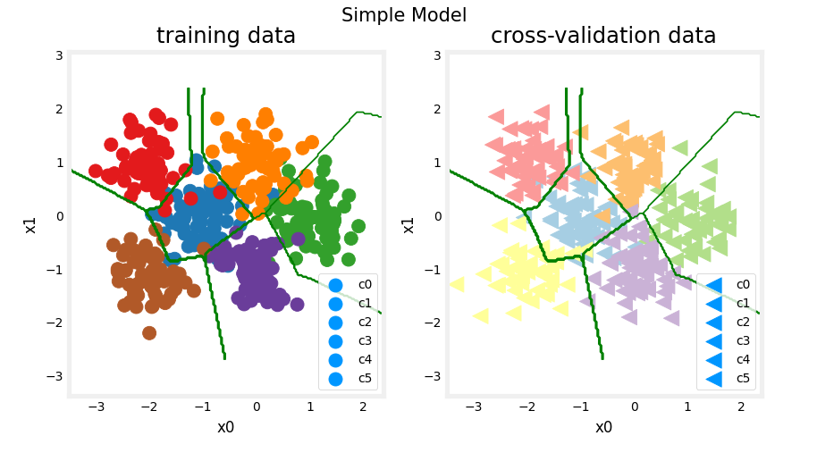
This simple models does pretty well. Let’s calculate the classification error.

training_cerr_simple = eval_cat_err(y_train, model_predict_s(X_train))
cv_cerr_simple = eval_cat_err(y_cv, model_predict_s(X_cv))
print(f"categorization error, training, simple model, {training_cerr_simple:0.3f}, complex model: {training_cerr_complex:0.3f}" )
print(f"categorization error, cv,       simple model, {cv_cerr_simple:0.3f}, complex model: {cv_cerr_complex:0.3f}" )

Output

categorization error, training, simple model, 0.062, complex model: 0.003
categorization error, cv,       simple model, 0.087, complex model: 0.122

Our simple model has a little higher classification error on training data but does better on cross-validation data than the more complex model.

6 - Regularization

As in the case of polynomial regression, one can apply regularization to moderate the impact of a more complex model. Let’s try this below.

Exercise 5

Reconstruct your complex model, but this time include regularization.
Below, compose a three-layer model:

• Dense layer with 120 units, relu activation, kernel_regularizer=tf.keras.regularizers.l2(0.1)
• Dense layer with 40 units, relu activation, kernel_regularizer=tf.keras.regularizers.l2(0.1)
• Dense layer with 6 units and a linear activation.
  Compile using
• loss with SparseCategoricalCrossentropy, remember to use from_logits=True
• Adam optimizer with learning rate of 0.01.

# UNQ_C5
# GRADED CELL: model_r

tf.random.set_seed(1234)
model_r = Sequential(
    [
        ### START CODE HERE ### 
        Dense(120, activation="relu", kernel_regularizer=tf.keras.regularizers.l2(0.1)),
        Dense(40, activation="relu", kernel_regularizer=tf.keras.regularizers.l2(0.1)),
        Dense(6, activation="linear")
        ### END CODE HERE ### 
    ], name= None
)
model_r.compile(
    ### START CODE HERE ### 
    loss=SparseCategoricalCrossentropy(from_logits=True),
    optimizer=Adam(0.01),
    ### END CODE HERE ### 
)

Unit Test

# BEGIN UNIT TEST
model_r.fit(
    X_train, y_train,
    epochs=1000
)
# END UNIT TEST

# BEGIN UNIT TEST
model_r.summary()

model_r_test(model_r, classes, X_train.shape[1]) 
# END UNIT TEST

Output

Model: "sequential"
_________________________________________________________________
 Layer (type)                Output Shape              Param #   
=================================================================
 dense_6 (Dense)             (None, 120)               360       
                                                                 
 dense_7 (Dense)             (None, 40)                4840      
                                                                 
 dense_8 (Dense)             (None, 6)                 246       
                                                                 
=================================================================
Total params: 5,446
Trainable params: 5,446
Non-trainable params: 0
_________________________________________________________________
ddd
All tests passed!

Hints

Summary should match this (layer instance names may increment )

Model: "ComplexRegularized"
_________________________________________________________________
Layer (type)                 Output Shape              Param #   
=================================================================
L1 (Dense)                   (None, 120)               360       
_________________________________________________________________
L2 (Dense)                   (None, 40)                4840      
_________________________________________________________________
L3 (Dense)                   (None, 6)                 246       
=================================================================
Total params: 5,446
Trainable params: 5,446
Non-trainable params: 0
_________________________________________________________________

More hints

tf.random.set_seed(1234)
model_r = Sequential(
    [
        Dense(120, activation = 'relu', kernel_regularizer=tf.keras.regularizers.l2(0.1), name="L1"), 
        Dense(40, activation = 'relu', kernel_regularizer=tf.keras.regularizers.l2(0.1), name="L2"),  
        Dense(classes, activation = 'linear', name="L3")  
    ], name="ComplexRegularized"
)
model_r.compile(
    loss=tf.keras.losses.SparseCategoricalCrossentropy(from_logits=True), 
    optimizer=tf.keras.optimizers.Adam(0.01),                             
)

model_r.fit(
    X_train,y_train,
    epochs=1000
)          

Plot

#make a model for plotting routines to call
model_predict_r = lambda Xl: np.argmax(tf.nn.softmax(model_r.predict(Xl)).numpy(),axis=1)
 
plt_nn(model_predict_r, X_train,y_train, classes, X_cv, y_cv, suptitle="Regularized")

Output

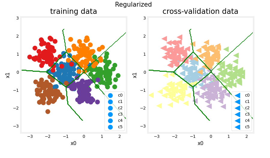
The results look very similar to the ‘ideal’ model. Let’s check classification error.

training_cerr_reg = eval_cat_err(y_train, model_predict_r(X_train))
cv_cerr_reg = eval_cat_err(y_cv, model_predict_r(X_cv))
test_cerr_reg = eval_cat_err(y_test, model_predict_r(X_test))
print(f"categorization error, training, regularized: {training_cerr_reg:0.3f}, simple model, {training_cerr_simple:0.3f}, complex model: {training_cerr_complex:0.3f}" )
print(f"categorization error, cv,       regularized: {cv_cerr_reg:0.3f}, simple model, {cv_cerr_simple:0.3f}, complex model: {cv_cerr_complex:0.3f}" )

Output

categorization error, training, regularized: 0.072, simple model, 0.062, complex model: 0.003
categorization error, cv,       regularized: 0.066, simple model, 0.087, complex model: 0.122

The simple model is a bit better in the training set than the regularized model but it worse in the cross validation set.

7 - Iterate to find optimal regularization value

As you did in linear regression, you can try many regularization values. This code takes several minutes to run. If you have time, you can run it and check the results. If not, you have completed the graded parts of the assignment!

tf.random.set_seed(1234)
lambdas = [0.0, 0.001, 0.01, 0.05, 0.1, 0.2, 0.3]
models=[None] * len(lambdas)
for i in range(len(lambdas)):
    lambda_ = lambdas[i]
    models[i] =  Sequential(
        [
            Dense(120, activation = 'relu', kernel_regularizer=tf.keras.regularizers.l2(lambda_)),
            Dense(40, activation = 'relu', kernel_regularizer=tf.keras.regularizers.l2(lambda_)),
            Dense(classes, activation = 'linear')
        ]
    )
    models[i].compile(
        loss=tf.keras.losses.SparseCategoricalCrossentropy(from_logits=True),
        optimizer=tf.keras.optimizers.Adam(0.01),
    )

    models[i].fit(
        X_train,y_train,
        epochs=1000
    )
    print(f"Finished lambda = {lambda_}")

Output

13/13 [==============================] - 0s 1ms/step - loss: 0.4242
Epoch 996/1000
13/13 [==============================] - 0s 1ms/step - loss: 0.4068
Epoch 997/1000
13/13 [==============================] - 0s 1ms/step - loss: 0.4396
Epoch 998/1000
13/13 [==============================] - 0s 1ms/step - loss: 0.4108
Epoch 999/1000
13/13 [==============================] - 0s 1ms/step - loss: 0.4226
Epoch 1000/1000
13/13 [==============================] - 0s 1ms/step - loss: 0.4581
Finished lambda = 0.3

Plot

plot_iterate(lambdas, models, X_train, y_train, X_cv, y_cv)

Output

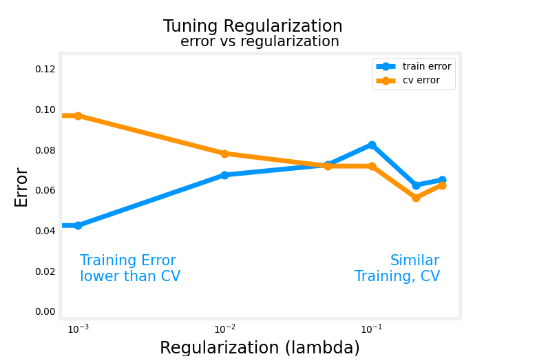
As regularization is increased, the performance of the model on the training and cross-validation data sets converge. For this data set and model, lambda > 0.01 seems to be a reasonable choice.

7.1 Test

Let’s try our optimized models on the test set and compare them to ‘ideal’ performance.

plt_compare(X_test,y_test, classes, model_predict_s, model_predict_r, centers)

Output

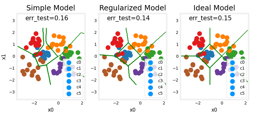
Our test set is small and seems to have a number of outliers so classification error is high. However, the performance of our optimized models is comparable to ideal performance.

Congratulations!

You have become familiar with important tools to apply when evaluating your machine learning models. Namely:

• splitting data into trained and untrained sets allows you to differentiate between underfitting and overfitting
• creating three data sets, Training, Cross-Validation and Test allows you to
  • train your parameters $W,B$ with the training set
  • tune model parameters such as complexity, regularization and number of examples with the cross-validation set
  • evaluate your ‘real world’ performance using the test set.
• comparing training vs cross-validation performance provides insight into a model’s propensity towards overfitting (high variance) or underfitting (high bias)

其他

commit

git commit -m "Finish xxx part of week xx of Advanced Learning Algorithms"

For example

git commit -m "Finish '[7] Skewed datasets (optional)' part of week 03 of Advanced Learning Algorithms"

\quad 是空格
\ 小空格
\; 中等空格

英文发音

intersect very few data points 和很少的点相交

hews very closely to every data point 非常接近每个数据点。

A polynomial model with degree 1 produces a straight line that intersects very few data points, while the maximum degree hews very closely to every data point.

harmonic mean 调和平均数

調和平均數（英語：harmonic mean），是求一組數值的平均數的方法中的一種，一般是在計算平均速率時使用。

調和平均數是將所有數值取倒數並求其算術平均數後，再將此算術平均數取倒數而得，其結果等於數值的個數除以數值倒數的總和。

来源：https://zh.wikipedia.org/zh-tw/%E8%B0%83%E5%92%8C%E5%B9%B3%E5%9D%87%E6%95%B0

threshold the output at 0.5 取0.5阈值

We would typically threshold the output of logistic regression at 0.5 and predict 1 if f of x is greater than equal to 0.5 and predict 0 if it’s less than 0.5.

左上角: upper left

左下角: lower left

by summing up this upper-left cell and this lower-left cell

Without consent and without disclosure 未经同意和免责声明

But clearly using this technology to
generate fake videos without consent and without disclosure would be unethical.

incendiary 助燃的，煽动性的，英 [ɪnˈsendiəri]

dark skinned individuals: 黑人

speak to the mobile phone

type into the mobile phone

speaking to your mobile phone rather than typing into your mobile phone.

panacea 万能药，万能之计 英 [ˌpænəˈsiːə]

give your learning algorithm performance a huge boost.

tempting 诱人的，有吸引力的，英 [ˈtemptɪŋ]

caveat警告，告诫 英 [ˈkæviæt]

skewed: 歪曲的;有偏颇的;不准确的;

go up, come down 增长，下降，反义词

接近xx : approach xx

increase training data, then the training error
will continue to go up, but then the cross-validation
error hopefully will come down and
approach J train.

in this high variance scenario： 在这种high variance（过拟合）的情况下

Throw more training data added: 添加更多的数据

That’s why before investing a lot of effort into collecting
more training data, it’s worth checking if your learning algorithm has high bias, because if it does, then you probably need to do some other things other than just throw more training data added.

be flat

flatten out = plateau 持平，达到平台

In fact, this curve of training error may start to flatten out. We call it plateau, meaning flatten out after a while.

完美拟合很难

it gets even a little bit harder to fit all of them perfectly

fit a quadratic model: 二阶函数模型

quadratic 英 [kwɒˈdrætɪk] 二次的

hone our intuition: 磨练（训练）我们的直觉

transcribe 英 [trænˈskraɪb]，转录，转换为xxx形式

diagnostic 英 [ˌdaɪəɡˈnɒstɪk] , 诊断的

10 to the power of 10: $10^{10}$

convex: 凹函数 ˌkänˈveks， 重音在后

e to the negative z: $e^{-z}$

square of xxx: xxx的平方

parabola: 抛物线， pəˈrabələ

backslash: 反斜线 \