Advanced Learning Algorithms Week 01

笔者在2022年7月份取得这门课的证书，现在（2024年2月25日）才想起来将笔记发布到博客上。
Website: https://www.coursera.org/learn/advanced-learning-algorithms?specialization=machine-learning-introduction

Offered by: DeepLearning.AI and Stanford

课程地址：https://www.coursera.org/learn/machine-learning

本笔记包含字幕，quiz的答案以及作业的代码，仅供个人学习使用，如有侵权，请联系删除。

This week, you’ll learn about neural networks and how to use it for classification tasks. You’ll use the TensorFlow framework to build a neural network with just a few lines of code. Then, dive deeper by learning how to code up your own neural network in Python, “from scratch”. Optionally, you can learn more about how neural network computations are implemented efficiently use parallel processing (vectorization).

Learning Objectives

---

• Get familiar with the diagram and components of a neural network
• Understand the concept of a “layer” in a neural network
• Understand how neural networks learn new features.
• Understand how activations are calculated at each layer.
• Learn how a neural network can perform classification on an image.
• Use a framework, TensorFlow, to build a neural network for classification of an image.
• Learn how data goes into and out of a neural network layer in TensorFlow
• Build a neural network in regular Python code (from scratch) to make predictions.
• (Optional): Learn how neural networks use parallel processing (vectorization) to make computations faster.

[01] Neural networks intuition

Welcome

Welcome to Course 2 of this machine learning
specialization. In this course, you’ll learn
about neural networks, also called deep
learning algorithms, as well as decision trees.

These are some of the most powerful and widely
used machine learning algorithms and you’d get to implement them and get
them to work for yourself.

One of the things you see
also in this course is practical advice on how to build machine
learning systems. This part of the material is
quite unique to this course.

When you’re building a practical
machine learning system, there are a lot of
decisions you have to make, such as should you
spend more time collecting data or should you buy a much bigger GPU to build a much bigger
neural network?

Even today, when I visit a leading tech
company and talk to the team working there on a machine learning
application, unfortunately, sometimes I look at what
they’ve been doing for the last six months and go, gee, someone could have
told you maybe even six months ago that that approach wasn’t
going to work that well.

With some of the tips that
you learn in this course, I hope that you’ll
be one or the ones to not waste those six
months, but instead, be able to make more systematic
and better decisions about how to build practical working machine
learning applications.

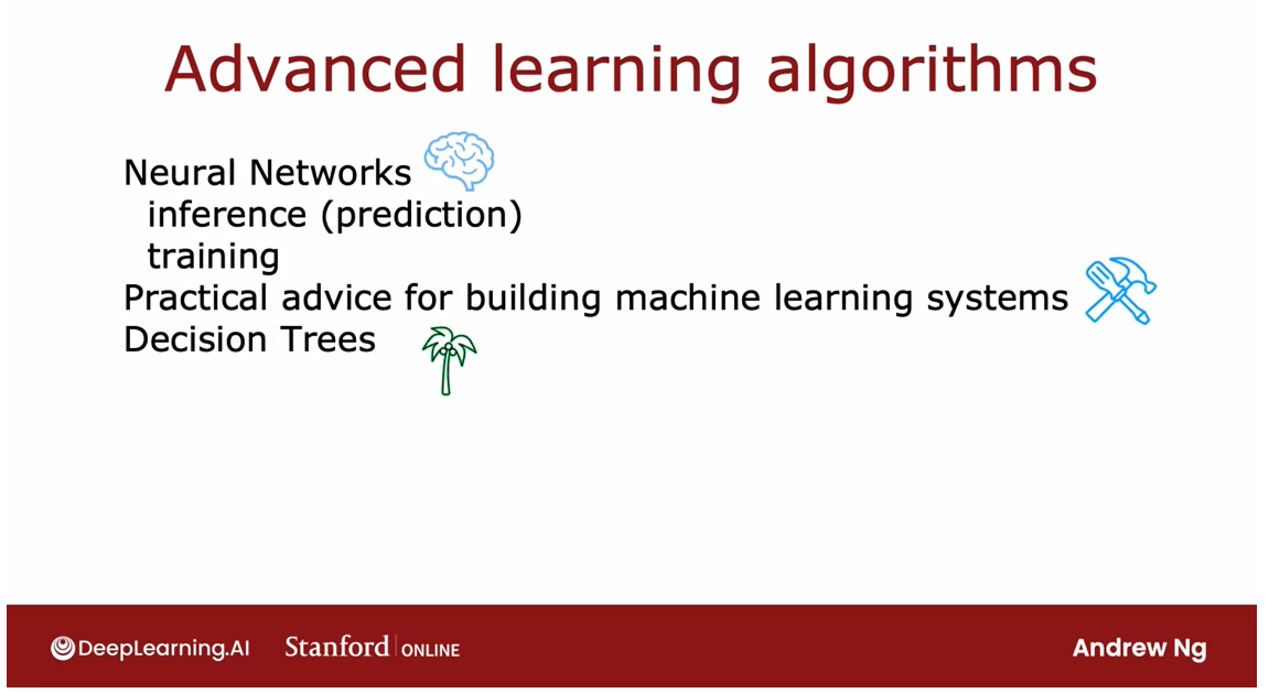
With that, let’s dive in. In detail, this is what you see in the four weeks
of this course.

In Week 1, we’ll go over
neural networks and how to carry out
inference or prediction.

If you were to go
to the Internet and download the parameters of a neural network that
someone else had trained and whose parameters that
posted on the Internet, then to use that
neural network to make predictions would be
called inference, and you learned how
neural networks work, and how to do inference
in this week.

Next week, you’ll learn how to train your own neural network. In particular, if you have a training set of
labeled examples, X and Y, how do you train the parameters of a neural
network for yourself?

In the third week, we’ll then go into
practical advice for building machine learning
systems and I’ll share with you some tips that I think even highly paid engineers building machine learning
systems very successfully today don’t really always manage
to consistently apply and I think that will help you build systems yourself
efficiently and quickly.

Then in the final
week of this course, you learn about decision trees.

While decision trees don’t get
as much buzz in the media, there’s local less hype about decision trees compared
to neural networks. They are also one of the widely used and very
powerful learning algorithms that I think there’s
a good chance you end up using yourself if you end
up building an application.

With that, let’s jump into neural networks and we’re going to start by taking a quick
look at how the human brain, that is how the
biological brain works. Let’s go on to the next video.

Neurons and the brain

Original motivation: mimic how the human brain or how the biological brain learns and thinks

When neural networks were first invented many decades ago, the original motivation was to write software that could mimic how the human brain or how the biological brain
learns and thinks.

Even though today,
neural networks, sometimes also called
artificial neural networks, have become very
different than how any of us might think about how the brain actually
works and learns.

Some of the biological
motivations still remain in the way we think about artificial neural networks or computer neural
networks today.

Let’s start by taking a
look at how the brain works and how that relates
to neural networks.

The human brain, or
maybe more generally, the biological brain demonstrates
a higher level or more capable level of
intelligence and anything else would be
on the bill so far. So neural networks
has started with the motivation of
trying to build software to mimic the brain.

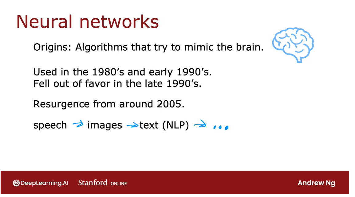
Work in neural networks had
started back in the 1950s, and then it fell out
of favor for a while.

Then in the 1980s
and early 1990s, they gained in popularity
again and showed tremendous traction
in some applications like handwritten
digit recognition, which were used
even backed then to read postal codes for routing mail and for reading dollar figures in
handwritten checks.

But then it fell out of favor
again in the late 1990s.

It was from about
2005 that it enjoyed a resurgence and also became re-branded little bit
with deep learning.

One of the things that
surprised me back then was deep learning and neural networks meant
very similar things.

But maybe under appreciated at the time that the
term deep learning, just sounds much better because it’s deep
and this learning. So that turned out
to be the brand that took off in the last decade
or decade and a half.

Since then, neural networks have revolutionized application
area after application area.

I think the first
application area that modern neural
networks or deep learning, had a huge impact on was
probably speech recognition, where we started to see much better speech
recognition systems due to modern deep learning
and authors such as [inaudible] and Geoff Hinton
were instrumental to this, and then it started to make
inroads into computer vision.

Sometimes people still speak of the ImageNet moments in 2012, and that was maybe a bigger
splash where then [inaudible] draw their imagination and had a big impact on
computer vision.

Then the next few years, it made us inroads into texts or into natural
language processing, and so on and so forth.

Now, neural networks are
used in everything from climate change to medical
imaging to online advertising.

So proudly, recommendations
and really lots of application areas
of machine learning now use neural networks.

Even though today’s
neural networks have almost nothing to do with
how the brain learns, there was the early
motivation of trying to build software
to mimic the brain.

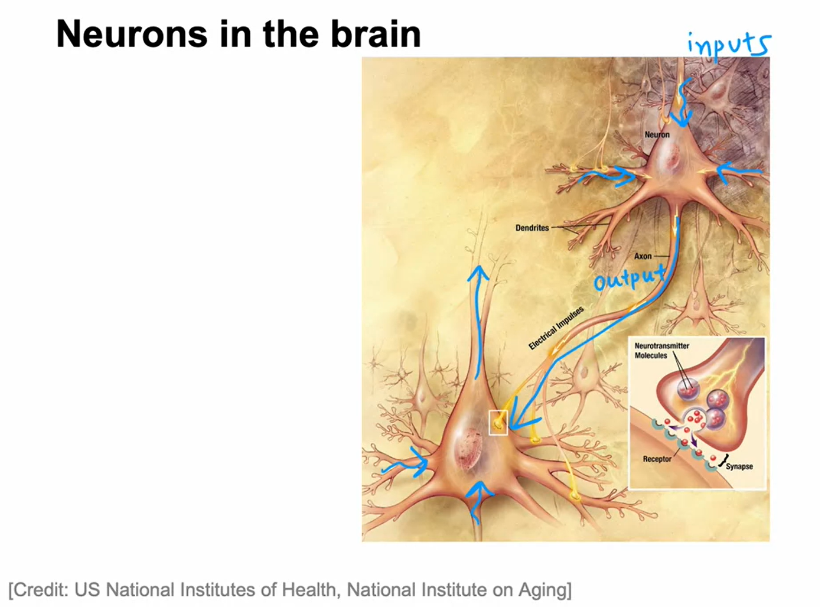
So how does the brain work?

Here’s a diagram illustrating what neurons in a
brain look like.

All of human thought is from neurons like this in
your brain and mine, sending electrical impulses and sometimes forming new
connections of other neurons.

The stuff of which human thought is made

Given a neuron like this one, it has a number of
inputs where it receives electrical impulses
from other neurons, and then this neuron that I’ve circled carries out
some computations and will then send this outputs to other neurons by this
electrical impulses, and this upper neuron’s
output in turn becomes the input to
this neuron down below, which again aggregates
inputs from multiple other neurons to then
maybe send its own output, to yet other neurons, and this is the stuff of
which human thought is made.

Here’s a simplified diagram
of a biological neuron.

Biological neuron:

nucleus of the neuron: 神经元核

dendrites: 树突 ˈdendrīt

axon：轴突 ˈakˌsän

A neuron comprises a cell
body shown here on the left, and if you have taken
a course in biology, you may recognize this to be
the nucleus of the neuron.

As we saw on the previous slide, the neuron has different inputs. In a biological neuron, the input wires are
called the dendrites, and it then occasionally
sends electrical impulses to other neurons via
the output wire, which is called the axon. Don’t worry about these
biological terms. If you saw them in
a biology class, you may remember them, but you don’t really need to memorize any of these terms for the purpose of building
artificial neural networks.

But this biological
neuron may then send electrical impulses that become the input to another neuron.

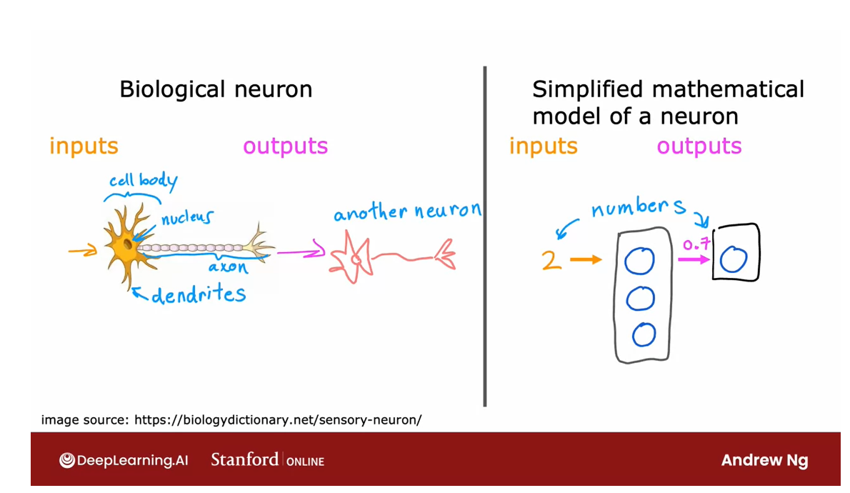
So the artificial
neural network uses a very simplified
Mathematical model of what a biological
neuron does.

I’m going to draw
a little circle here to denote a single neuron.

What a neuron does is
it takes some inputs, one or more inputs, which are just numbers. It does some computation and it outputs
some other number, which then could be an
input to a second neuron, shown here on the right.

Neurons in neural network: input a few numbers, carry out some computation, and output some other numbers.

When you’re building an
artificial neural network or deep learning algorithm, rather than building
one neuron at a time, you often want to simulate many such
neurons at the same time. In this diagram, I’m
drawing three neurons.

What these neurons do collectively is
input a few numbers, carry out some computation, and output some other numbers.

Now, at this point, I’d like to give one big caveat, which is that even though I made a loose analogy between biological neurons and
artificial neurons, I think that today we have almost no idea how the
human brain works.

In fact, every few years, neuroscientists make some
fundamental breakthrough about how the brain works. I think we’ll continue to do so for the foreseeable future.

That to me is a
sign that there are many breakthroughs
that are yet to be discovered about how the
brain actually works, and thus attempts to blindly mimic what we know of
the human brain today, which is frankly very little, probably won’t get us that far toward building
raw intelligence.

Certainly not with
our current level of knowledge in neuroscience. Having said that, even with these extremely simplified
models of a neuron, which we’ll talk about,
we’ll be able to build really powerful deep
learning algorithms.

So as you go deeper into neural networks and
into deep learning, even though the origins were
biologically motivated, don’t take the biological
motivation too seriously.

In fact, those of us that do research in deep learning have shifted away from looking to biological motivation that much. But instead, they’re just using engineering principles to figure out how to build algorithms
that are more effective.

But I think it might still
be fun to speculate and think about how
biological neurons work every now and then.

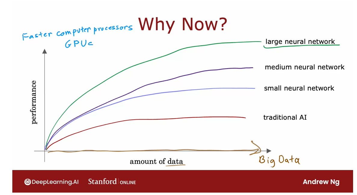
Why is it that only in the last handful of years that neural networks have really taken off?

The ideas of neural
networks have been around for many decades. A few people have asked me, “Hey Andrew, why now? Why is it that only
in the last handful of years that neural networks
have really taken off?”

This is a picture I draw for them when I’m
asked that question and that maybe you could draw for others as well if they
ask you that question.

Draw a picture:

• horizontal axis: the amount of data
• vertical axis: the performance (or the accuracy) of a learning algorithm

Let me plot on the
horizontal axis the amount of data you
have for a problem, and on the vertical axis, the performance or
the accuracy of a learning algorithm
applied to that problem.

In many application areas, the amount of digital data has exploded.

Over the last couple of decades, with the rise of the Internet, the rise of mobile phones, the digitalization
of our society, the amount of data
we have for a lot of applications has steadily
marched to the right.

Lot of records that
use P on paper, such as if you order something rather than it being
on a piece of paper, there’s much more likely
to be a digital record. Your health record,
if you see a doctor, is much more likely
to be digital now compared to on
pieces of paper.

So in many application areas, the amount of digital
data has exploded.

Traditional learning algorithm: won’t be able to scale with the amount of data

Meaning: Even if you fed those algorithms more data, it was very difficult to get the performance to keep on going up.

What we saw was with traditional machine-learning
algorithms, such as logistic regression
and linear regression, even as you fed those
algorithms more data, it was very difficult to get the performance to
keep on going up.

So it was as if the traditional learning
algorithms like linear regression and
logistic regression, they just weren’t able to scale with the amount of data
we could now feed it and they weren’t able to
take effective advantage of all this data we had for
different applications.

Train neural network with different size

What AI researchers
started to observe was that if you were to train a small neural network
on this dataset, then the performance
maybe looks like this.

If you were to train a
medium-sized neural network, meaning one with
more neurons in it, its performance may
look like that.

If you were to train a
very large neural network, meaning one with a lot of
these artificial neurons, then for some applications the performance will
just keep on going up.

So this meant two things, it meant that for
a certain class of applications where you
do have a lot of data, sometimes you hear the
term big data toss around, if you’re able to train a very large neural
network to take advantage of that huge amount
of data you have, then you could attain
performance on anything ranging from speech recognition,
to image recognition, to natural language processing
applications and many more, they just were not possible with earlier generations of
learning algorithms.

This caused deep learning
algorithms to take off, and this too is why faster
computer processes, including the rise of GPUs
or graphics processor units.

This is hardware
originally designed to generate nice-looking
computer graphics, but turned out to be really powerful for deep
learning as well.

That was also a major force in allowing deep
learning algorithms to become what it is today.

That’s how neural
networks got started, as well as why they took off so quickly in the
last several years. Let’s now dive more deeply into the details of how neural
network actually works. Please go on to the next video.

Demand Prediction

To illustrate how
neural networks work, let’s start with an example.

We’ll use an example from demand prediction in which you look at the product
and try to predict, will this product be
a top seller or not? Let’s take a look.

Predict a product is a top seller or not

In this example, you’re
selling T-shirts and you would like to know if a particular T-shirt
will be a top seller, yes or no, and you
have collected data of different t-shirts that
were sold at different prices, as well as which ones
became a top seller.

Used by retailers today

This type of application is used by retailers today in order to plan better inventory levels as well as marketing campaigns. If you know what’s likely to be a top seller, you would plan, for example, to just purchase more of that
stock in advance.

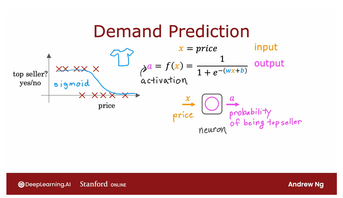
In this example,
the input feature x is the price of the T-shirt, and so that’s the input to
the learning algorithm.

If you apply logistic
regression to fit a sigmoid function to the data that might
look like that then the outputs of your prediction
might look like this, 1/1 plus e to the
negative wx plus b.

Previously, we had
written this as f of x as the output of
the learning algorithm.

In order to set us up to
build a neural network, I’m going to switch the
terminology a little bit and use the alphabet a to denote the output of this logistic
regression algorithm.

The term a stands
for activation, and it’s actually a
term from neuroscience, and it refers to how
much a neuron is sending a high output to other
neurons downstream from it.

It turns out that this logistic regression units or this little logistic
regression algorithm, can be thought of as a very simplified model of a
single neuron in the brain.

Where what the neuron does is it takes us
input the price x, and then it computes
this formula on top, and it outputs the number a, which is computed
by this formula, and it outputs the probability of this T-shirt
being a top seller.

Another way to think
of a neuron is as a tiny little computer whose only job is to input
one number or a few numbers, such as a price, and then
to output one number or maybe a few other
numbers which in this case is the probability of the T-shirt
being a top seller.

As I alluded in the
previous video, a logistic regression
algorithm is much simpler than what any biological neuron in your
brain or mine does. Which is why the artificial
neural network is such a vastly oversimplified
model of the human brain.

Even though in
practice, as you know, deep learning algorithms
do work very well.

Given this description
of a single neuron, building a neural network now it just requires taking a bunch of these neurons and wiring them together or putting
them together.

Let’s now look at a
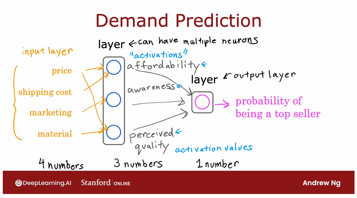
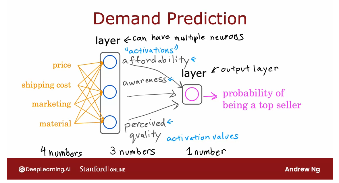
more complex example of demand prediction.

In this example, we’re
going to have four features to predict whether or not
a T-shirt is a top seller. The features are the
price of the T-shirt, the shipping costs, the amounts of marketing of that
particular T-shirt, as well as the material quality, is this a high-quality, thick cotton versus maybe
a lower quality material?

Now, you might suspect
that whether or not a T-shirt becomes a top seller actually depends
on a few factors.

First, one is the
affordability of this T-shirt.

Second is, what’s the degree of awareness of this T-shirt
that potential buyers have?

Third is perceived quality to bias or potential bias saying this is a
high-quality T-shirt.

What I’m going to do is create
one artificial neuron to try to estimate the
probability that this T-shirt is perceive
as highly affordable.

Affordability is mainly a
function of price and shipping costs because the
total amount of the pay is some of the price
plus the shipping costs.

We’re going to use a
little neuron here, a logistic regression unit
to input price and shipping costs and predict do people
think this is affordable?

Second, I’m going to create another artificial
neuron here to estimate, is there high awareness of this? Awareness in this case is mainly a function of the
marketing of the T-shirt.

Finally, going to create
another neuron to estimate do people perceive
this to be of high quality, and that may mainly
be a function of the price of the T-shirt and
of the material quality.

Price is a factor here because fortunately
or unfortunately, if there’s a very
high priced T-shirt, people will sometimes perceive that to be of high
quality because it is very expensive than maybe people think it’s going
to be of high-quality.

Given these estimates of
affordability, awareness, and perceived quality we
then wire the outputs of these three neurons to another
neuron here on the right, that then there’s another
logistic regression unit.

That finally inputs
those three numbers and outputs the probability of this t-shirt being a top seller. In the terminology
of neural networks, we’re going to group these three neurons together
into what’s called a layer.

A layer is a grouping
of neurons which takes us input the same
or similar features, and that in turn outputs
a few numbers together.

These three neurons on the left form one layer which is why I drew them
on top of each other, and this single neuron on
the right is also one layer. The layer on the left
has three neurons, so a layer can have multiple
neurons or it can also have a single neuron as in the case of this
layer on the right.

This layer on the
right is also called the output layer
because the outputs of this final neuron is the output probability predicted
by the neural network.

Activation: refer to the degree that the biological neuron is sending a high output value (or sending many electronical impulses) to other neurons to the downstream from it.

In the terminology of neural networks we’re
also going to call affordability
awareness and perceive quality to be activations.

The term activations comes
from biological neurons, and it refers to the degree that the biological
neuron is sending a high output value or sending many electrical impulses to other neurons to the
downstream from it.

These numbers on
affordability, awareness, and perceived quality are the activations of these
three neurons in this layer, and also this output
probability is the activation of this neuron
shown here on the right.

This particular neural network therefore carries out
computations as follows.

It inputs four numbers then this layer of the
neural network uses those four numbers to compute the new numbers also
called activation values.

Then the final layer, the output layer of the
neural network used those three numbers to
compute one number.

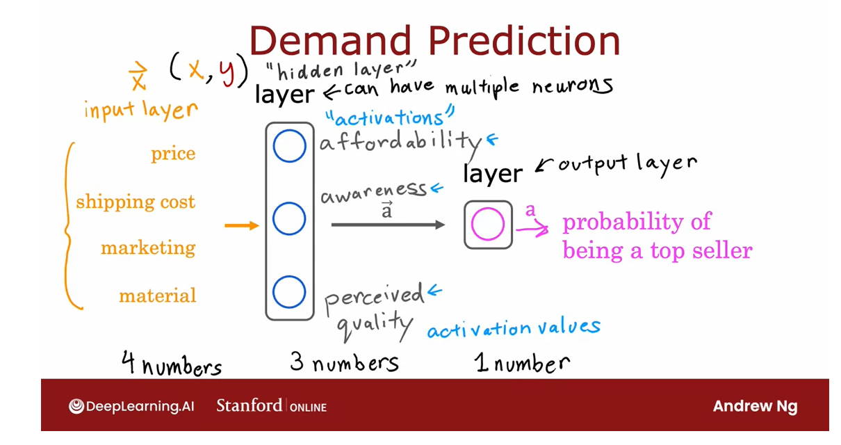
In a neural network this list of four numbers is also
called the input layer, and that’s just a
list of four numbers. Now, there’s one simplification I’d like make to
this neural network.

The way I’ve
described it so far, we had to go through the
neurons one at a time and decide what inputs it would
take from the previous layer.

For example, we said
affordability is a function of just price and shipping
costs and awareness is a function of just
marketing and so on, but if you’re building
a large neural network it’d be a lot of work
to go through and manually decide which neurons should take which
features as inputs.

Difficult to go through and manually decide which neurons should take which features as inputs.

In practice: layer in the middle will have access to every feature, to every value from the previous layer.

The way a neural network
is implemented in practice each neuron
in a certain layer;

say this layer in the middle, will have access
to every feature, to every value from
the previous layer, from the input layer which is
why I’m now drawing arrows from every input
feature to every one of these neurons shown
here in the middle.

You can imagine that if
you’re trying to predict affordability and it knows what’s the price shipping
cost marketing and material, may be you’ll learn to ignore marketing and material
and just figure out through setting the
parameters appropriately to only focus on the subset
of features that are most relevant to affordability.

Input features comprise feature vector

To further simplify
the notation and the description of this
neural network I’m going to take these four
input features and write them as a vector x, and we’re going to view the
neural network as having four features that comprise
this feature vector x.

This feature vector is
fed to this layer in the middle which then computes
three activation values. That is these numbers and these three activation values in turn becomes
another vector which is fed to this final
output layer that finally outputs the probability of this t-shirt to
being a top seller. That’s all a neural network is.

It has a few layers
where each layer inputs a vector and outputs
another vector of numbers.

For example, this layer
in the middle inputs four numbers x and outputs three numbers
corresponding to affordability, awareness, and
perceived quality.

To add a little bit
more terminology, you’ve seen that this
layer is called the output layer and this layer is
called the input layer. To give the layer in the
middle a name as well, this layer in the middle
is called a hidden layer. I know that this is
maybe not the best or the most intuitive name but that terminology comes from that’s when you have
a training set.

In a training set, you get to observe both x and y. Your data set tells you
what is x and what is y, and so you get data that tells you what are the correct inputs
and the correct outputs.

But your dataset
doesn’t tell you what are the correct values
for affordability, awareness, and
perceived quality. The correct values
for those are hidden.

You don’t see them
in the training set, which is why this layer in the middle is called
a hidden layer.

I’d like to share with you
another way of thinking about neural networks
that I’ve found useful for building my
intuition about it.

Cover up the left half of the diagram

Just let me cover up the
left half of this diagram, and see what we’re left with.

What you see here
is that there is a logistic regression
algorithm or logistic regression unit
that is taking as input, affordability, awareness, and perceived
quality of a t-shirt, and using these three
features to estimate the probability of the
t-shirt being a top seller. This is just
logistic regression.

But the cool thing about this is rather than using
the original features, price, shipping cost,
marketing, and so on, is using maybe better set of features,
affordability, awareness, and perceived quality,
that are hopefully more predictive of whether or not this t-shirt will
be a top seller.

One way to think of this neural network is logistic regression: learn its own features

One way to think of
this neural network is, just logistic regression. But as a version of
logistic regression, they can learn its
own features that makes it easier to make
accurate predictions.

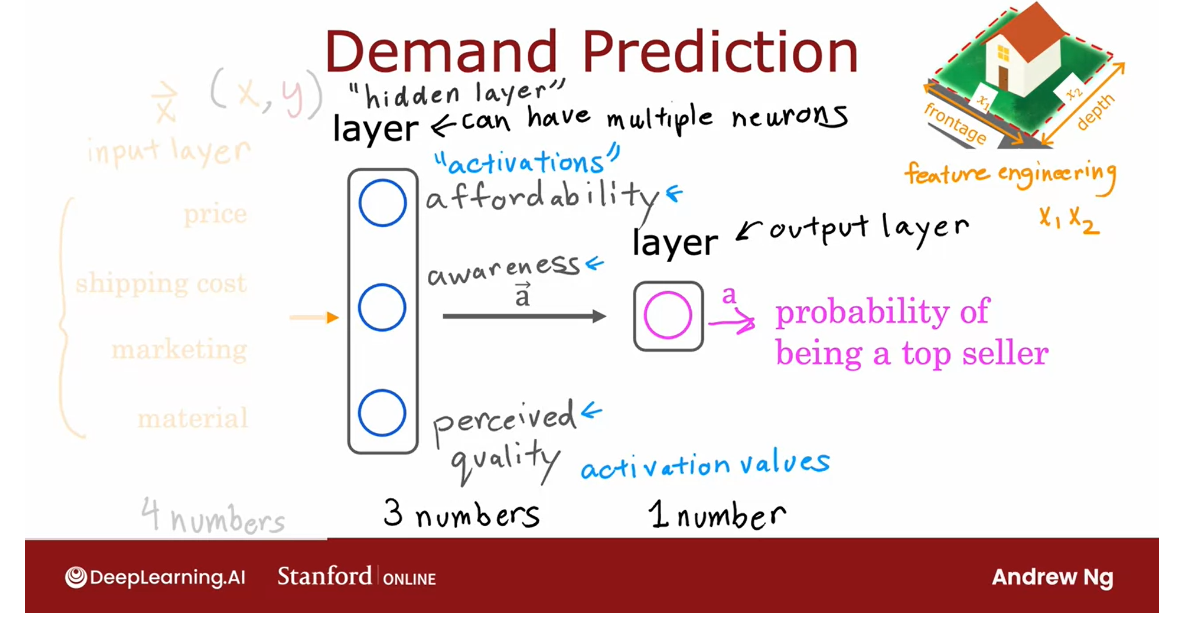
In fact, you might remember
from the previous week, this housing example
where we said that if you want to predict
the price of the house, you might take the frontage or the width of lots
and multiply that by the depth of a
lot to construct a more complex feature, x_1 times x_2, which was the size of the lawn.

There we were doing manual
feature engineering where we had to look
at the features x_1 and x_2 and decide by
hand how to combine them together to come up
with better features.

What the neural network
does is instead of you needing to manually
engineer the features, it can learn, as
you’ll see later, its on features to make the learning problem
easier for itself. This is what makes neural networks one of the most powerful learning
algorithms in the world today.

To summarize, a neural network, does this, the input layer
has a vector of features, four numbers in this example, it is input to the hidden layer, which outputs three numbers.

I’m going to use a
vector to denote this vector of activations that this hidden layer outputs.

Then the output layer
takes its input to three numbers and
outputs one number, which would be the
final activation, or the final prediction
of the neural network.

Property of neural network: don’t need to go in to explicitly decide what features the NN should compute

One note, even
though I previously described this neural network
as computing affordability, awareness, and
perceived quality, one of the really nice
properties of a neural network is when you train it from data, you don’t need to go in to explicitly decide
what other features, such as affordability and so on, that the neural network should compute instead or
figure out all by itself what are the features it wants to use in
this hidden layer.

That’s what makes it such a
powerful learning algorithm.

You’ve seen here one example
of a neural network and this neural network has a single layer that
is a hidden layer.

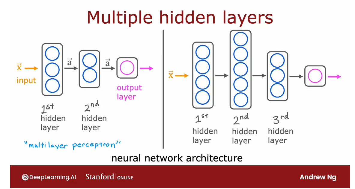
Let’s take a look at
some other examples of neural networks,
specifically, examples with more
than one hidden layer. Here’s an example.

This neural network has an input feature vector X that is fed to one hidden layer. I’m going to call this
the first hidden layer.

If this hidden layer
has three neurons, it will then output a vector
of three activation values.

These three numbers can then be input to the second
hidden layer.

If the second hidden layer has two neurons to logistic units, then this second
hidden there will output another vector of now two activation values
that maybe goes to the output layer that then outputs the neural
network’s final prediction.

Here’s another example. Here’s a neural network that it’s input goes to
the first hidden layer, the output of the
first hidden layer goes to the second hidden layer, goes to the third hidden layer, and then finally to
the output layer.

The architecture of the neural network: how many hidden layers and how many neurons per hidden layer is.

When you’re building
your own neural network, one of the decisions
you need to make is how many hidden layers do you want and how many neurons do you want each hidden
layer to have.

This question of how
many hidden layers and how many neurons
per hidden layer is a question of the architecture
of the neural network.

You’ll learn later in
this course some tips for choosing an appropriate
architecture for a neural network.

But choosing the right number of hidden layers and number of hidden units per layer can have an impact on the performance of a learning algorithm as well.

Later in this course,
you’ll learn how to choose a good architecture for your
neural network as well.

Neural network with multi layers: Multilayer perceptron 多层感知机

By the way, in some
of the literature, you see this type of
neural network with multiple layers like this
called a multilayer perceptron.

If you see that, that just
refers to a neural network that looks like what you’re
seeing here on the slide. That’s a neural network.

I know we went through
a lot in this video. Thank you for sticking with me. But you now know how a
neural network works.

In the next video, let’s take a look
at how these ideas can be applied to other
applications as well. In particular, we’ll
take a look at the computer vision application
of face recognition. Let’s go on to the next video.

Example: Recognizing Images

In the last video, you saw how a neural network works in a
demand prediction example.

Let’s take a look at how you
can apply a similar type of idea to computer vision
application.

Let’s dive in. If you’re building a face
recognition application, you might want to train a neural network that takes
as input a picture like this and outputs the identity of the person in the picture.

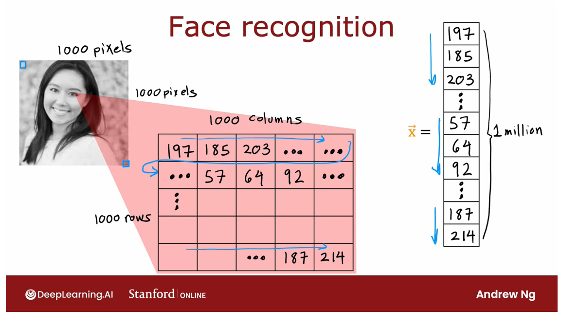
This image is 1,000
by 1,000 pixels. Its representation
in the computer is actually as 1,000 by 1,000 grid, or also called 1,000 by 1,000 matrix of pixel
intensity values.

In this example, my
pixel intensity values or pixel brightness values, goes from 0-255 and so 197 here would be the brightness of the pixel in the very upper
left of the image, 185 is brightness of the
pixel, one pixel over, and so on down to 214 would be the lower
right corner of this image.

Take pixel intensity values and unroll them into a vector

NN: Takes as input a feature vector with xxx pixel brightness values

NN: Output the identity of a person in the picture

If you were to take these pixel intensity values and unroll them into a vector, you end up with a
list or a vector of a million pixel
intensity values. One million because 1,000 by 1,000 square gives you
a million numbers. The face recognition problem is, can you train a neural network that takes as input a
feature vector with a million pixel
brightness values and outputs the identity of
the person in the picture.

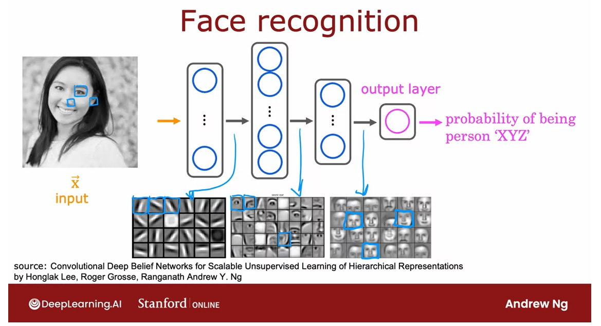
This is how you might build a neural network to
carry out this task.

The input image X is fed
to this layer of neurons. This is the first hidden layer, which then extract
some features.

The upwards of this
first hidden layer is fed to a second hidden layer and that output is fed to a third layer and then
finally to the upper layer, which then estimates, say the probability of this
being a particular person.

Peer at the different neurons in the hidden layers to figure out what they may be computing.

One interesting
thing would be if you look at a neural network
that’s been trained on a lot of images of
faces and to try to visualize what are these hidden layers,
trying to compute.

It turns out that when you train a system like this
on a lot of pictures of faces and you peer at the different neurons
in the hidden layers to figure out what they may be computing this is
what you might find.

In the first hidden layer: Neurons are looking for very short lines or edges

In the first hidden layer, you might find one
neuron that is looking for the low vertical line or
a vertical edge like that.

A second neuron looking for a oriented line or
oriented edge like that.

The third neuron
looking for a line at that orientation, and so on.

In the earliest layers
of a neural network, you might find that the
neurons are looking for very short lines or very
short edges in the image.

In the second hidden layer: Learn to group lots of short lines to look for parts of faces.

If you look at the
next hidden layer, you find that these neurons
might learn to group together lots of little short lines and little short edge segments in order to look for
parts of faces.

For example, each of these
little square boxes is a visualization of what that
neuron is trying to detect.

This first neuron
looks like it’s trying to detect the presence or absence of an eye in a certain
position of the image.

The second neuron,
looks like it’s trying to detect like a corner of a nose and maybe
this neuron over here is trying to detect
the bottom of a nose.

Then as you look
at the next hidden layer in this example, the neural network
is aggregating different parts of faces to then try to detect presence
or absence of larger, coarser face shapes.

Then finally, detecting how much the face corresponds to
different face shapes creates a rich set of features
that then helps the output layer try to determine the identity
of the person picture.

NN: feature detectors at the different hidden layers learn all by themselves.

A remarkable thing about the neural network
is you can learn these feature detectors at the different hidden
layers all by itself.

In this example, no
one ever told it to look for short little
edges in the first layer, and eyes and noses
and face parts in the second layer and then more complete face shapes
at the third layer.

The neural network is able
to figure out these things all by itself from data.

Just one note, in
this visualization, the neurons in the
first hidden layer are shown looking at relatively small windows
to look for these edges.

In the second hidden layer
is looking at bigger window, and the third hidden layer is looking at even bigger window.

These little neurons
visualizations actually correspond
to differently sized regions in the image.

Just for fun, let’s see
what happens if you were to train this neural network
on a different dataset, say on lots of pictures of cars, picture on the side. The same learning algorithm
is asked to detect cars, will then learn edges
in the first layer.

Pretty similar but then they’ll learn to detect parts of cars in the second hidden
layer and then more complete car shapes in
the third hidden layer.

Just by feeding it
different data, the neural network
automatically learns to detect very different features
so as to try to make the predictions
of car detection or person recognition
or whether there’s a particular given task
that is trained on.

That’s how a neural
network works for computer vision application.

In fact, later this week, you’ll see how you can build a neural network
yourself and apply it to a handwritten digit
recognition application.

So far we’ve been going
over the description of intuitions of neural networks to give you a feel
for how they work. In the next video, let’s look more deeply into
the concrete mathematics and a concrete implementation
of details of how you actually build one or more
layers of a neural network, and therefore how
you can implement one of these things yourself. Let’s go on to the next video.

[02] Practice quiz: Neural networks intuition

Practice quiz: Neural networks intuition

Latest Submission Grade 100%

[03] Neural network model

Neural network layer

The fundamental
building block of most modern neural networks
is a layer of neurons.

In this video, you’ll
learn how to construct a layer of neurons and
once you have that down, you’d be able to take those
building blocks and put them together to form a
large neural network.

Let’s take a look at how
a layer of neurons works.

Here’s the example we had from the demand prediction
example where we had four input features
that were set to this layer of three neurons
in the hidden layer that then sends its output to this output layer
with just one neuron.

Let’s zoom in to the hidden layer to look
at its computations.

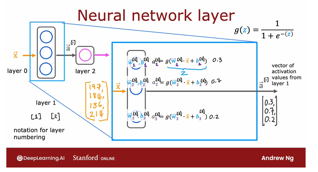
This hidden layer
inputs four numbers and these four numbers are inputs
to each of three neurons.

Each of these three neurons
is just implementing a little logistic
regression unit or a little bit logistic
regression function.

Take this first neuron. It has two parameters, w and b. In fact, to denote that, this is the first hidden unit, I’m going to subscript
this as w_1, b_1.

What it does is I’ll output
some activation value a, which is g of w_1 in a
product with x plus b_1, where this is the
familiar z value that you have learned about in logistic regression in
the previous course, and g of z is the familiar
logistic function, 1 over 1 plus e to
the negative z.

Maybe this ends up
being a number 0.3 and that’s the activation value
a of the first neuron.

To denote that this
is the first neuron, I’m also going to add a
subscript a_1 over here, and so a_1 may be
a number like 0.3.

There’s a 0.3 chance of this being highly affordable
based on the input features.

Now let’s look at
the second neuron.

The second neuron has
parameters w_2 and b_2, and these w, b or w_2, b_2 are the parameters of
the second logistic unit.

It computes a_2 equals the
logistic function g applied to w_2 dot product x plus b_2 and this may be some
other number, say 0.7. Because in this example, there’s a 0.7 chance that we think the potential buyers
will be aware of this t-shirt.

Similarly, the third neuron has a third set of
parameters w_3, b_3.

Similarly, it computes an activation value
a_3 equals g of w_3 dot product x plus b_3
and that may be say, 0.2.

In this example, these
three neurons output 0.3, 0.7, and 0.2, and this vector of three numbers becomes the vector of
activation values a, that is then passed to the final output layer
of this neural network.

Give the layers different numbers

Now, when you build neural networks with
multiple layers, it’ll be useful to give the
layers different numbers.

By convention, this layer
is called layer 1 of the neural network
and this layer is called layer 2 of
the neural network.

The input layer
is also sometimes called layer 0 and today, there are neural
networks that can have dozens or even
hundreds of layers.

But in order to
introduce notation to help us distinguish
between the different layers, I’m going to use
superscript square bracket 1 to index into
different layers.

In particular, a superscript in square brackets
1, I’m going to use, that’s a notation to
denote the output of layer 1 of this hidden layer
of this neural network, and similarly, w_1, b_1 here are the parameters of the first unit in layer
1 of the neural network, so I’m also going to add a superscript in
square brackets 1 here, and w_2, b_2 are the parameters of the second hidden unit or the second hidden
neuron in layer 1.

Its parameters are also
denoted here w¹ like so.

Similarly, I can add superscripts square
brackets like so to denote that these are the activation values of the hidden units of layer
1 of this neural network.

I know maybe this notation is getting a little
bit cluttered.

But the thing to
remember is whenever you see this superscript
square bracket 1, that just refers to a quantity that is associated with layer
1 of the neural network.

If you see superscript
square bracket 2, that refers to a quantity
associated with layer 2 of the neural network and similarly for
other layers as well, including layer 3, layer 4 and so on for neural
networks with more layers.

That’s the computation of layer
1 of this neural network. Its output is this
activation vector, a² and I’m going to
copy this over here because this output a_1
becomes the input to layer 2.

Now let’s zoom into the computation of layer
2 of this neural network, which is also the output layer. The input to layer 2 is
the output of layer 1, so a_1 is this vector 0.3, 0.7, 0.2 that we just computed on the previous
part of this slide.

Because the output layer
has just a single neuron, all it does is it
computes a_1 that is the output of this first
and only neuron, as g, the sigmoid function
applied to w _1 in a product with a³, so this is the input
into this layer, and then plus b_1.

Here, this is the quantity
z that you familiar with and g as before is the sigmoid function
that you apply to this. If this results in
a number, say 0.84, then that becomes the output
layer of the neural network.

In this example, because the output layer has
just a single neuron, this output is just a scalar, is a single number rather
than a vector of numbers.

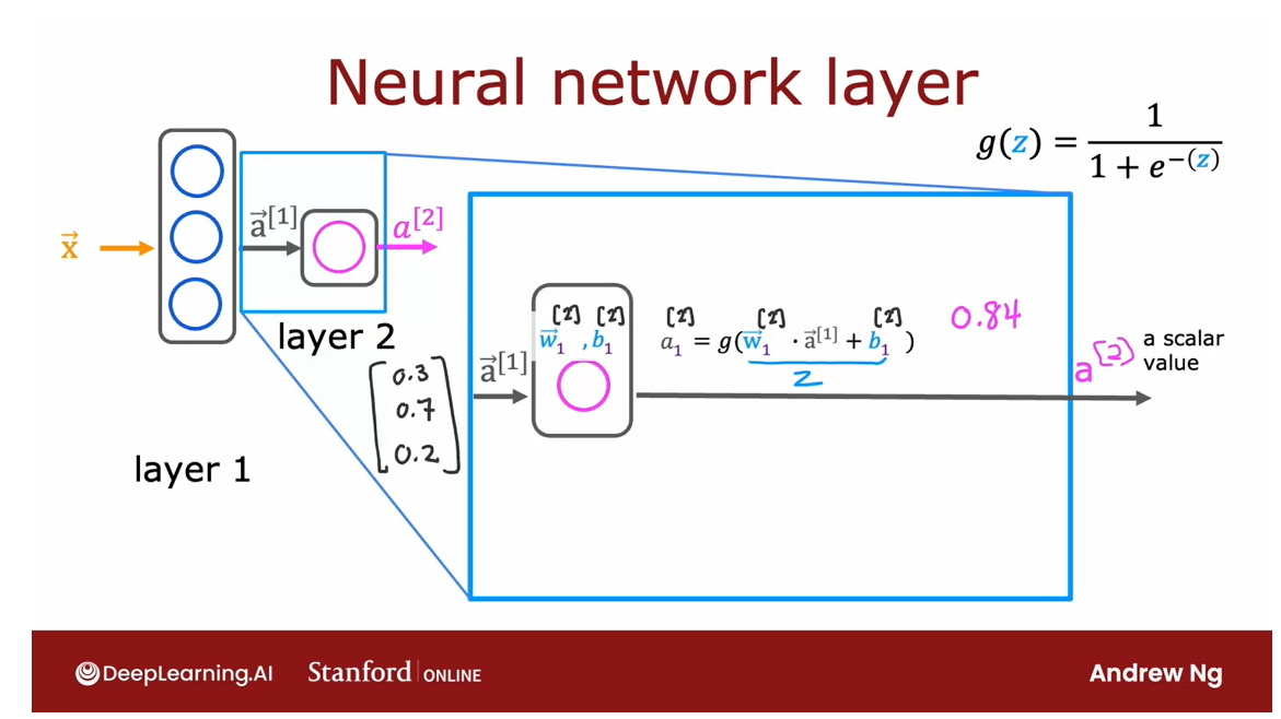
Sticking with our notational
convention from before, we’re going to use a superscript
in square brackets 2, to denote the quantities associated with layer 2
of this neural network, so a⁴ is the
output of this layer, and so I’m going
to also copy this here as the final output
of the neural network.

To make the notation consistent, you can also add these
superscripts square bracket 2s to denote that these are the parameters and
activation values associated with layer 2
of the neural network.

Once the neural network
has computed a_2, there’s one final
optional step that you can choose to implement or not, which is if you want
a binary prediction, 1 or 0, is this a top seller? Yes or no? As you
can take the number a superscript square
brackets 2 subscript 1, and this is the number
0.84 that we computed, and threshold this at 0.5. If it’s greater than 0.5, you can predict y hat equals 1 and if it
is less than 0.5, then predict your
y hat equals 0.

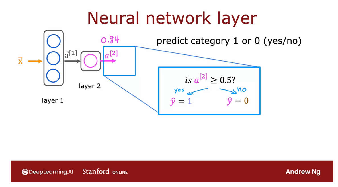
We saw this thresholding as
well when you learned about logistic regression in the first course of
the specialization. If you wish, this then gives you the final prediction y hat
as either one or zero, if you don’t want
just the probability of it being a top seller. So that’s how a
neural network works.

Every layer inputs a
vector of numbers and applies a bunch of logistic
regression units to it, and then computes
another vector of numbers that then
gets passed from layer to layer until you get to the final output
layers computation, which is the prediction
of the neural network.

Then you can either
threshold at 0.5 or not to come up with
the final prediction.

With that, let’s go on to
use this foundation we’ve built now to look at
some even more complex, even larger neural
network models. I hope that by seeing
more examples, this concept of layers
and how to put them together to build
a neural network will become even clearer. So let’s go on to
the next video.

More complex neural networks

In the last video, you learned about the neural
network layer and how that takes this inputs a
vector of numbers and in turn, outputs another
vector of numbers.

In this video, let’s use that layer to build a more
complex neural network.

Through this, I hope that the notation that
we’re using for neural networks
will become clearer and more concrete as
well. Let’s take a look.

Four layers

This is the running example that I’m going to use throughout this video as an example of a more complex
neural network.

This network has four layers, not counting the input layer, which is also called Layer 0, where layers 1, 2, and 3 are hidden layers, and Layer 4 is the output layer, and Layer 0, as usual, is the input layer.

By convention, when we say that a neural network
has four layers, that includes all the hidden
layers in the output layer, but we don’t count
the input layer. This is a neural network
with four layers in the conventional way of
counting layers in the network.

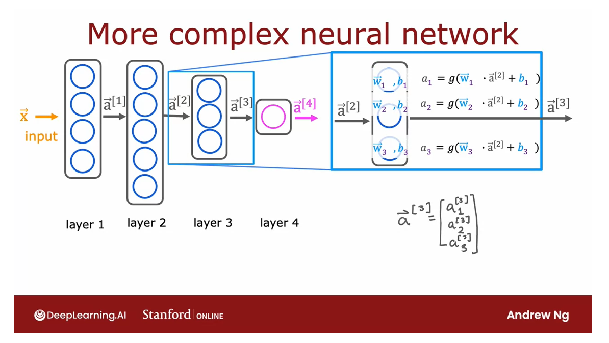
Let’s zoom in to Layer 3, which is the third and
final hidden layer to look at the computations
of that layer.

Layer 3 inputs a vector, a superscript square bracket 2 that was computed by
the previous layer, and it outputs a_3, which is another vector.

What is the computation that
Layer 3 does in order to go from a_2 to a_3?

If it has three neurons or we
call it three hidden units, then it has parameters w_1, b_1, w_2, b_2, and w_3, b_3 and it computes a_1
equals sigmoid of w_1. product with this input
to the layer plus b_1, and it computes a_2
equals sigmoid of w_2. product with again a_2, the input to the layer plus
b_2 and so on to get a_3.

Then the output of this layer is a vector comprising a_1, a_2, and a_3.

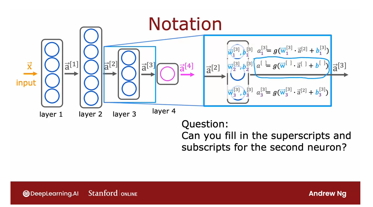
Again, by convention, if we want to more explicitly denote
that all of these are quantities associated
with Layer 3 then we add in all of
these superscript, square brackets 3 here, to denote that these parameters w and b are the parameters
associated with neurons in Layer 3 and that these activations are
activations with Layer 3.

Notice that this term here is w_1 superscript
square bracket 3, meaning the parameters
associated with Layer 3. product with a superscript
square bracket 2, which was the output of Layer 2, which became the
input to Layer 3.

That’s why it has a_3
here because it’s a parameter associator of
Layer 3. product with, and there’s a_2 there because
is the output of Layer 2.

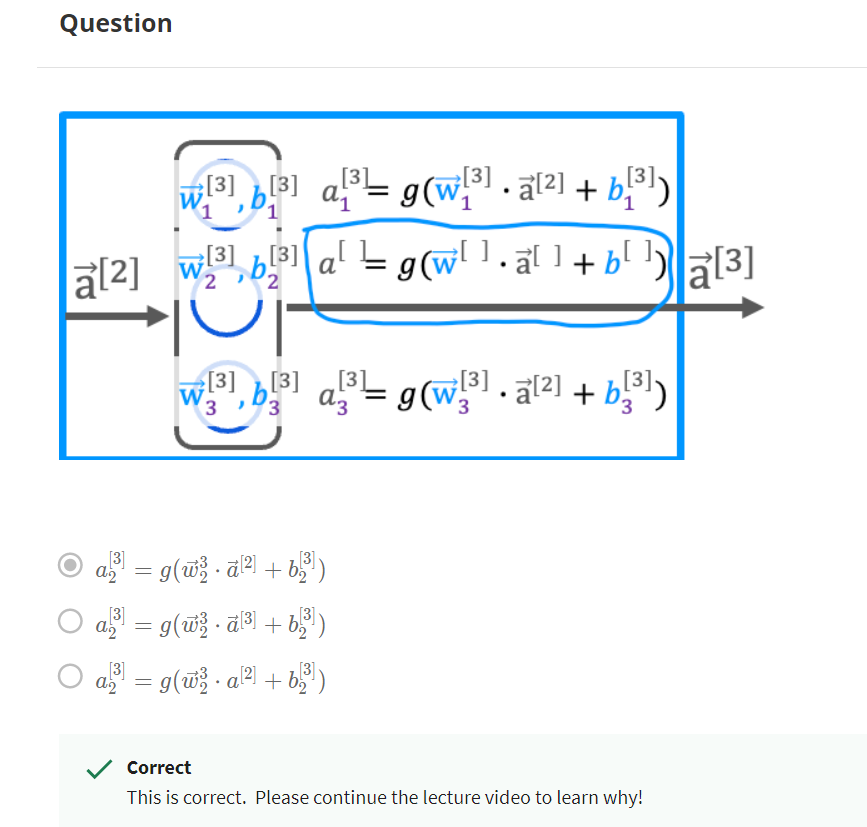
Now, let’s just do a quick double check on
our understanding of this. I’m going to hide the
superscripts and subscripts associated with
the second neuron and without rewinding
this video, go ahead and rewind if you want, but prefer you not.

But without rewinding
this video, are you able to think
through what are the missing superscripts and subscripts in this equation
and fill them in yourself?

Once you take a look at the end video quiz and
see if you can figure out what are the appropriate
superscripts and subscripts for this
equation over here.

To recap, a_3 is activation associated
with Layer 3 for the second neuron hence, this a_2 is a parameter
associated with the third layer.

For the second neuron, this is a_2, same as above and then plus b_3 too. Hopefully,
that makes sense.

Just the more general
form of this equation for an arbitrary Layer 0 and
for an arbitrary unit j, which is that a deactivation
outputs of layer l, unit j, like a32, that’s going to be
the sigmoid function applied to this term, which is the wave
vector of layer l, such as Layer 3 for the jth
unit so there’s a_2 again, in the example
above, and so that’s dot-producted with a
deactivation value.

Notice, this is not l, this is l minus 1, like a_2 above here
because you’re dot-producting with
the output from the previous layer
and then plus b, the parameter for this
layer for that unit j.

This gives you the activation
of layer l unit j, where the superscript in
square brackets l denotes layer l and a subscript
j denotes unit j.

When building neural networks, unit j refers to the jth neuron, so we use those
terms a little bit interchangeably where each unit is a single neuron in the layer.

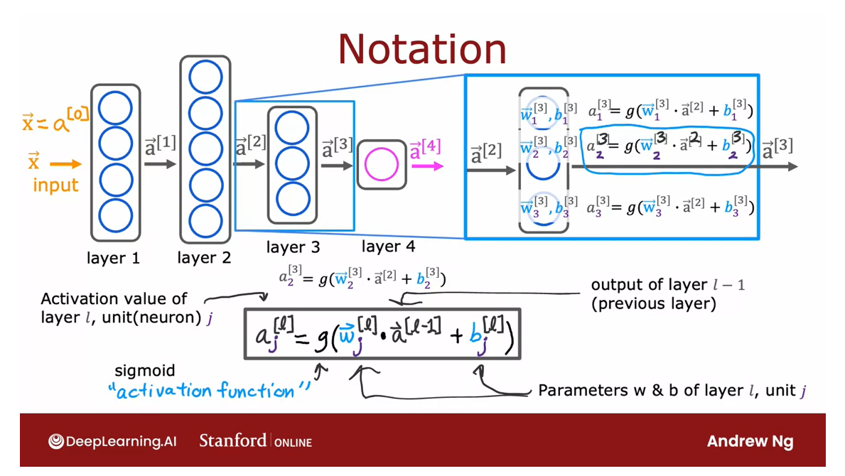
Activation function: outputs activation value

G here is the sigmoid function. In the context of
a neural network, g has another name, which is also called the
activation function, because g outputs this
activation value.

When I say activation function, I mean this function g here.

So far, the only activation
function you’ve seen, this is a sigmoid
function but next week, we’ll look at when
other functions, then the sigmoid function can be plugged in place of g as well…

The activation function
is just that function that outputs these
activation values.

Just one last piece of notation. In order to make all this
notation consistent, I’m also going to give the input vector X and
another name which is a_0, so this way, the same equation also works for the first layer, where when l is equal to 1, the activations of
the first layer, that is a_1, would be the sigmoid times the weights
dot-product with a_0, which is just this
input feature vector X.

With this notation, you
now know how to compute the activation values
of any layer in a neural network
as a function of the parameters as well as the activations of
the previous layer.

You now know how to
compute the activations of any layer given the activations
of the previous layer.

Let’s put this into an inference algorithm
for a neural network. In other words, how to get a neural network to
make predictions. Let’s go see that
in the next video.

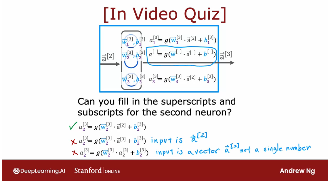
Quiz

Can you fill in the superscripts and subscripts for the second neuron?

answer

Inference: making predictions (forward propagation)

Let’s take what we’ve learned and put it
together into an algorithm to let your neural network make inferences or
make predictions.

Forward propagation

This will be an algorithm
called forward propagation. Let’s take a look.

Binary classification

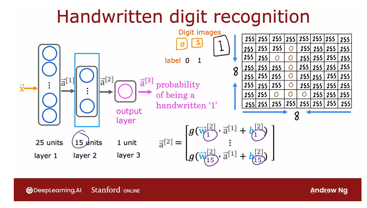
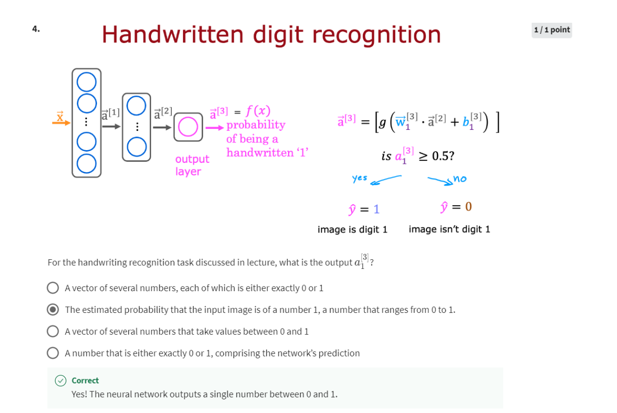
I’m going to use as a motivating example,
handwritten digit recognition.

And for simplicity we are just
going to distinguish between the handwritten digits zero and one.

So it’s just a binary classification
problem where we’re going to input an image and classify,
is this the digit zero or the digit one?

And you get to play with this yourself
later this week in the practice lab as well.

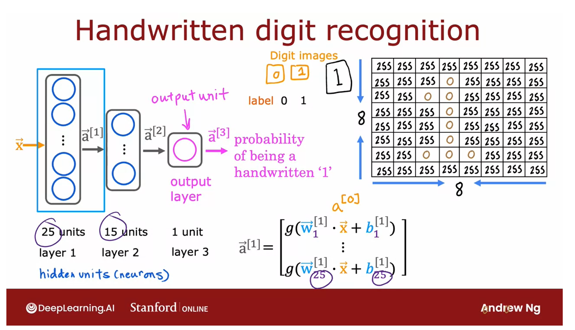
For the example of the slide,
I’m going to use an eight by eight image. And so this image of a one is this grid or
matrix of eight by eight or 64 pixel intensity values where 255
denotes a bright white pixel and zero would denote a black pixel.

And different numbers
are different shades of gray in between the shades of black and white.

Given these 64 input features, we’re going to use the neural
network with two hidden layers.

Where the first hidden layer
has 25 neurons or 25 units.

Second hidden layer has 15 neurons or
15 units.

And then finally the output layer or
outputs unit, what’s the chance of
this being 1 versus 0?.

So let’s step through the sequence
of computations that in your neural network will need to
make to go from the input X, this eight by eight or 64 numbers
to the predicted probability a3.

The first computation is
to go from X to a1, and that’s what the first layer of
the first hidden layer does.

It carries out a computation of
a super strip square bracket 1 equals this formula on the right.

Notice that a one has 25 numbers
because this hidden layer has 25 units. Which is why the parameters go from w1
through w25 as well as b1 through b25.

And I’ve written x here but I could also
have written a0 here because by convention the activation of layer zero, that is a0
is equal to the input feature value x.

So let’s just compute a1.

The next step is to compute a2. Looking at the second hidden layer, it then carries out this womputation
where a2 is a function of a1 and it’s computed as the safe point
activation function applied to w dot product a1 plus
the corresponding value of b.

Notice that layer two has 15 neurons or
15 units, which is why the parameters Here run
from w1 through w15 and b1 through b15. Now we’ve computed a2.

The Final step is then to compute a3 and
we do so using a very similar computation. Only now, this third layer,
the output layer has just one unit, which is why there’s just one output here.

So a3 is just a scalar. And finally you can optionally
take a3 subscript one and threshold it at 4.5 to come up with
a binary classification label. Is this the digit 1? Yes or no? So the sequence of computations first
takes x and then computes a1, and then computes a2, and then computes a3, which
is also the output of the neural networks.

You can also write that as f(x). So remember when we learned about linear
regression and logistic regression, we use f(x) to denote the output of
linear regression or logistic regression.

So we can also use f(x)
to denote the function computed by the neural
network as a function of x.

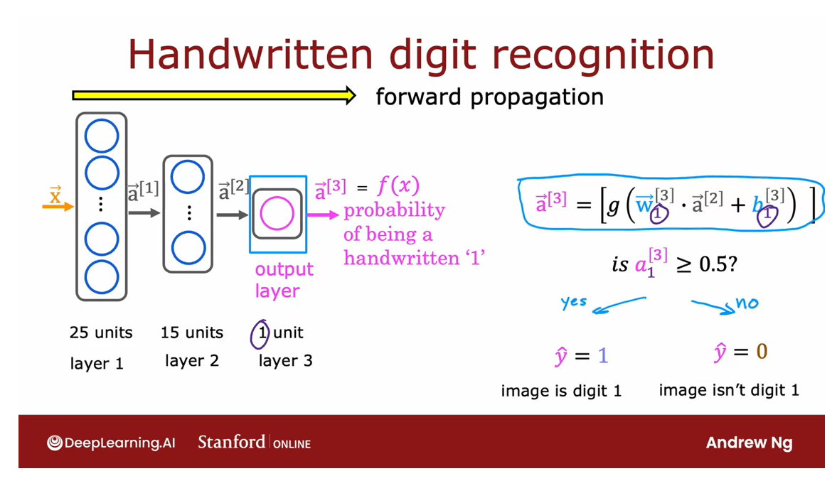
Computation goes from left to right: propagating the activations of the neurons

Because this computation goes from left to
right, you start from e and compute a1, then a2, then a3. This album is also called forward
propagation because you’re propagating the activations
of the neurons.

So you’re making these computations in
the four directions from left to right.

And this is in contrast to a different
algorithm called backward propagation or back propagation,
which is used for learning. And that’s something you
learn about next week.

NN architecture: the number of hidden units decreases as you get closer to the output layer

And by the way, this type of neural
network architecture where you have more hidden units initially and then the number of hidden units decreases
as you get closer to the output layer.

There’s also a pretty typical choice when
choosing neural network architectures. And you see more examples of this
in the practice lab as well.

So that’s neural network inference using
the forward propagation algorithm.

And with this, you’d be able to download
the parameters of a neural network that someone else had trained and
posted on the Internet. And you’d be able to carry out
inference on your new data using their neural network.

Now that you’ve seen the math and
the algorithm, let’s take a look at how you can
actually implement this in tensorflow. Specifically, let’s take a look
at this in the next video.

Lab: Neurons and Layers

Examples of Neurons and Layers

Optional Lab - Neurons and Layers

In this lab we will explore the inner workings of neurons/units and layers. In particular, the lab will draw parallels to the models you have mastered in Course 1, the regression/linear model and the logistic model. The lab will introduce Tensorflow and demonstrate how these models are implemented in that framework.

Packages

Tensorflow and Keras
Tensorflow is a machine learning package developed by Google. In 2019, Google integrated Keras into Tensorflow and released Tensorflow 2.0. Keras is a framework developed independently by François Chollet that creates a simple, layer-centric interface to Tensorflow. This course will be using the Keras interface.

import numpy as np
import matplotlib.pyplot as plt
import tensorflow as tf
from tensorflow.keras.layers import Dense, Input
from tensorflow.keras import Sequential
from tensorflow.keras.losses import MeanSquaredError, BinaryCrossentropy
from tensorflow.keras.activations import sigmoid
from lab_utils_common import dlc
from lab_neurons_utils import plt_prob_1d, sigmoidnp, plt_linear, plt_logistic
plt.style.use('./deeplearning.mplstyle')
import logging
logging.getLogger("tensorflow").setLevel(logging.ERROR)
tf.autograph.set_verbosity(0)

Neuron without activation - Regression/Linear Model

DataSet

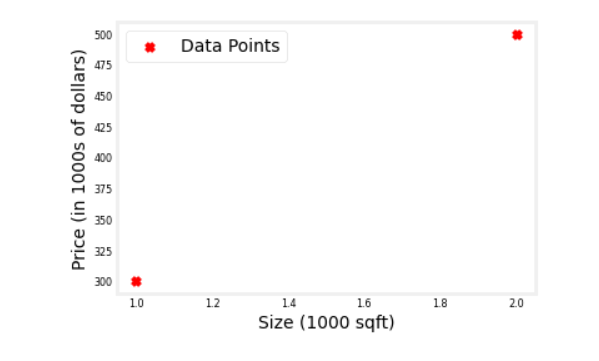
We’ll use an example from Course 1, linear regression on house prices.

X_train = np.array([[1.0], [2.0]], dtype=np.float32)           #(size in 1000 square feet)
Y_train = np.array([[300.0], [500.0]], dtype=np.float32)       #(price in 1000s of dollars)

fig, ax = plt.subplots(1,1)
ax.scatter(X_train, Y_train, marker='x', c='r', label="Data Points")
ax.legend( fontsize='xx-large')
ax.set_ylabel('Price (in 1000s of dollars)', fontsize='xx-large')
ax.set_xlabel('Size (1000 sqft)', fontsize='xx-large')
plt.show()

Output

Regression/Linear Model

The function implemented by a neuron with no activation is the same as in Course 1, linear regression:
$$f_{\mathbf{w},b}(x^{(i)})=\mathbf{w}\cdot x^{(i)}+b\text{\hspace{1em}(1)}$$

We can define a layer with one neuron or unit and compare it to the familiar linear regression function.

Let’s examine the weights.

linear_layer = tf.keras.layers.Dense(units=1, activation = 'linear', )
linear_layer.get_weights()

There are no weights as the weights are not yet instantiated. Let’s try the model on one example in X_train. This will trigger the instantiation of the weights. Note, the input to the layer must be 2-D, so we’ll reshape it.

a1 = linear_layer(X_train[0].reshape(1,1))
print(a1)

Output

这里的 1.39 是 w的值，是随机初始化得到的，而 b的初始值为0，这并并没有给出

tf.Tensor([[1.39]], shape=(1, 1), dtype=float32)

The result is a tensor (another name for an array) with a shape of (1,1) or one entry.
Now let’s look at the weights and bias. These weights are randomly initialized to small numbers and the bias defaults to being initialized to zero.

w, b= linear_layer.get_weights()
print(f"w = {w}, b={b}")

Output

w = [[1.39]], b=[0.]

A linear regression model (1) with a single input feature will have a single weight and bias. This matches the dimensions of our linear_layer above.

The weights are initialized to random values so let’s set them to some known values.

set_w = np.array([[200]])
set_b = np.array([100])

# set_weights takes a list of numpy arrays
linear_layer.set_weights([set_w, set_b])
print(linear_layer.get_weights())

Output

[array([[200.]], dtype=float32), array([100.], dtype=float32)]

Let’s compare equation (1) to the layer output.

a1 = linear_layer(X_train[0].reshape(1,1))
print(a1)
alin = np.dot(set_w,X_train[0].reshape(1,1)) + set_b
print(alin)

Output

tf.Tensor([[300.]], shape=(1, 1), dtype=float32)
[[300.]]

They produce the same values!
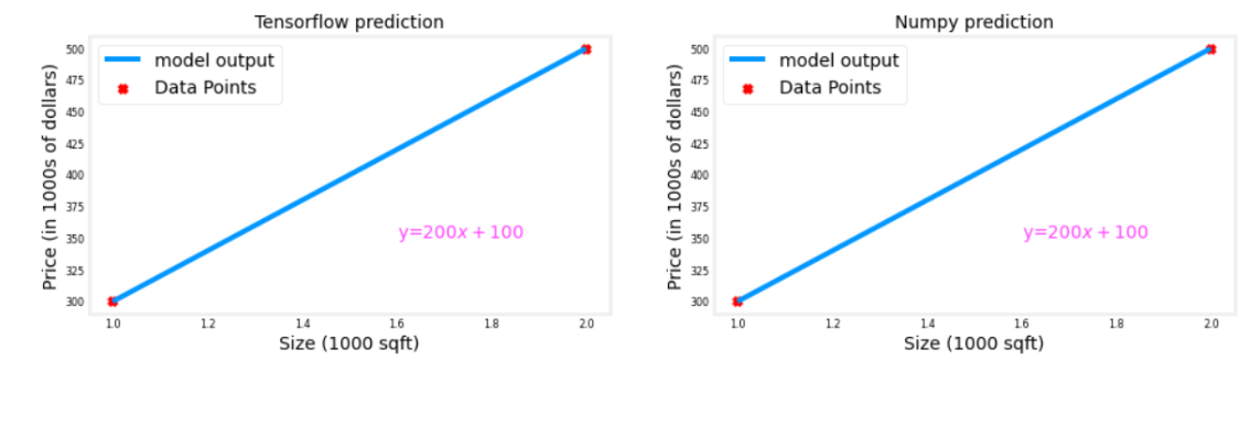
Now, we can use our linear layer to make predictions on our training data.

prediction_tf = linear_layer(X_train)
prediction_np = np.dot( X_train, set_w) + set_b

plt_linear(X_train, Y_train, prediction_tf, prediction_np)

Output

Neuron with Sigmoid activation

The function implemented by a neuron/unit with a sigmoid activation is the same as in Course 1, logistic regression:
$$f_{\mathbf{w},b}(x^{(i)})=g(\mathbf{w}{x}^{(i)}+b)\text{\hspace{1em}(2)}$$

where

$$g(x)=sigmoid(x)$$

Let’s set $w$ and $b$ to some known values and check the model.

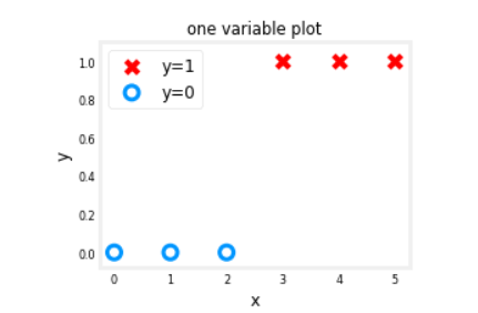
DataSet

We’ll use an example from Course 1, logistic regression.

X_train = np.array([0., 1, 2, 3, 4, 5], dtype=np.float32).reshape(-1,1)  # 2-D Matrix
Y_train = np.array([0,  0, 0, 1, 1, 1], dtype=np.float32).reshape(-1,1)  # 2-D Matrix


pos = Y_train == 1
neg = Y_train == 0
X_train[pos]

Output

array([3., 4., 5.], dtype=float32)

pos = Y_train == 1
neg = Y_train == 0

fig,ax = plt.subplots(1,1,figsize=(4,3))
ax.scatter(X_train[pos], Y_train[pos], marker='x', s=80, c = 'red', label="y=1")
ax.scatter(X_train[neg], Y_train[neg], marker='o', s=100, label="y=0", facecolors='none', 
              edgecolors=dlc["dlblue"],lw=3)

ax.set_ylim(-0.08,1.1)
ax.set_ylabel('y', fontsize=12)
ax.set_xlabel('x', fontsize=12)
ax.set_title('one variable plot')
ax.legend(fontsize=12)
plt.show()

Output

Logistic Neuron

We can implement a ‘logistic neuron’ by adding a sigmoid activation. The function of the neuron is then described by (2) above.
This section will create a Tensorflow Model that contains our logistic layer to demonstrate an alternate method of creating models. Tensorflow is most often used to create multi-layer models. The Sequential model is a convenient means of constructing these models.

model = Sequential(
    [
        tf.keras.layers.Dense(1, input_dim=1,  activation = 'sigmoid', name='L1')
    ]
)

model.summary() shows the layers and number of parameters in the model. There is only one layer in this model and that layer has only one unit. The unit has two parameters, $w$ and $b$.

model.summary()

Output

Model: "sequential_1"
_________________________________________________________________
 Layer (type)                Output Shape              Param #   
=================================================================
 L1 (Dense)                  (None, 1)                 2         
                                                                 
=================================================================
Total params: 2
Trainable params: 2
Non-trainable params: 0
_________________________________________________________________

logistic_layer = model.get_layer('L1')
w,b = logistic_layer.get_weights()
print(w,b)
print(w.shape,b.shape)

Output

[[1.19]] [0.]
(1, 1) (1,)

Let’s set the weight and bias to some known values.

set_w = np.array([[2]])
set_b = np.array([-4.5])
# set_weights takes a list of numpy arrays
logistic_layer.set_weights([set_w, set_b])
print(logistic_layer.get_weights())

Output

[array([[2.]], dtype=float32), array([-4.5], dtype=float32)]

Let’s compare equation (2) to the layer output.

a1 = model.predict(X_train[0].reshape(1,1))
print(a1)
alog = sigmoidnp(np.dot(set_w,X_train[0].reshape(1,1)) + set_b)
print(alog)

Output

[[0.01]]
[[0.01]]

They produce the same values!
Now, we can use our logistic layer and NumPy model to make predictions on our training data.

plt_logistic(X_train, Y_train, model, set_w, set_b, pos, neg)

Output

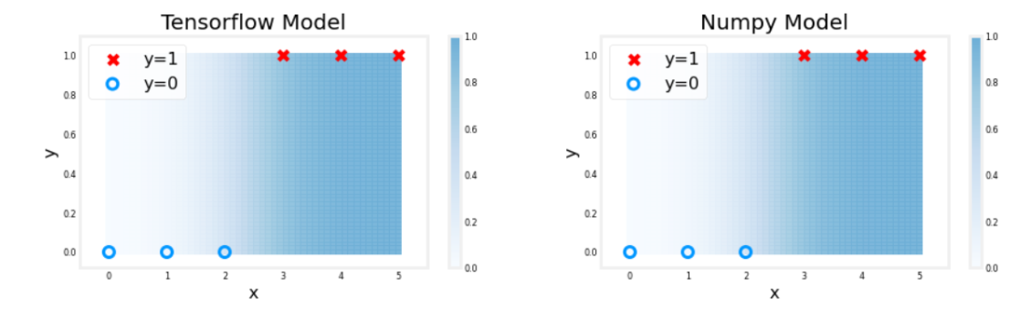
The shading above reflects the output of the sigmoid which varies from 0 to 1.

Congratulations!

You built a very simple neural network and have explored the similarities of a neuron to the linear and logistic regression from Course 1.

[04] Practice quiz: Neural network model

Practice quiz: Neural network model

Latest Submission Grade 93.75%

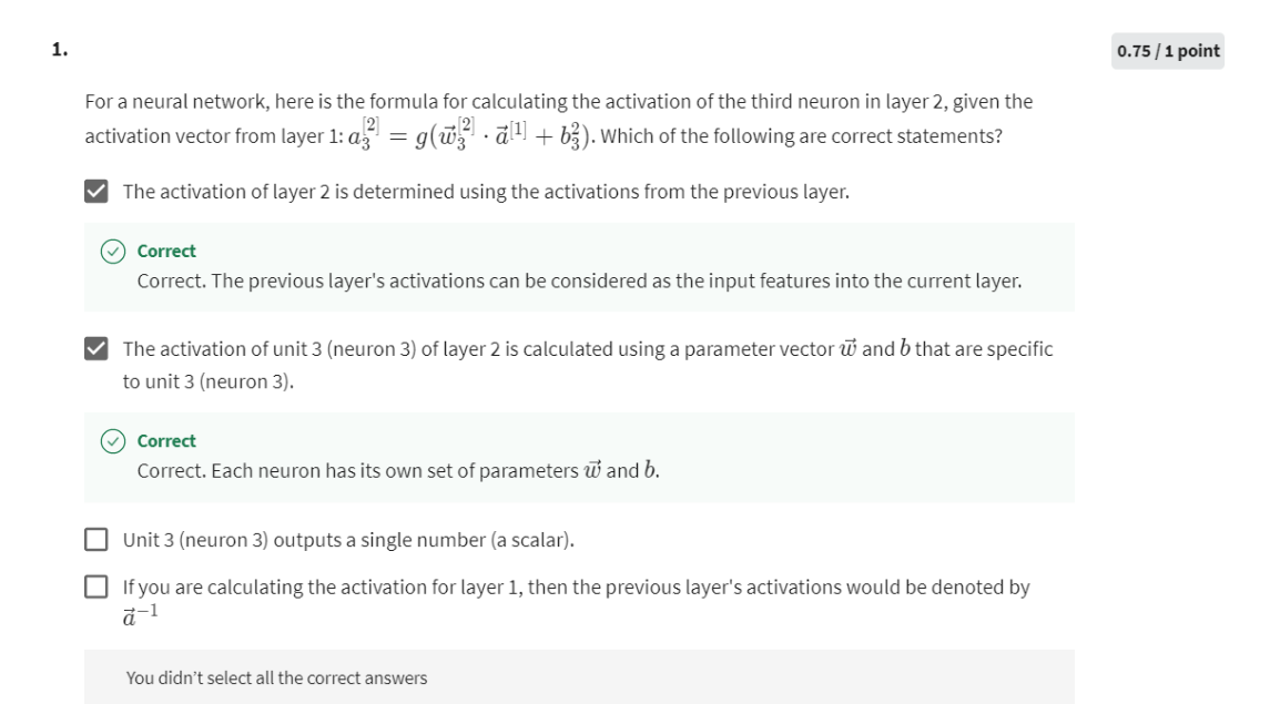
第一题第三个也要选的， Unit3 outputs a single number (a scalar) 这句话是对的

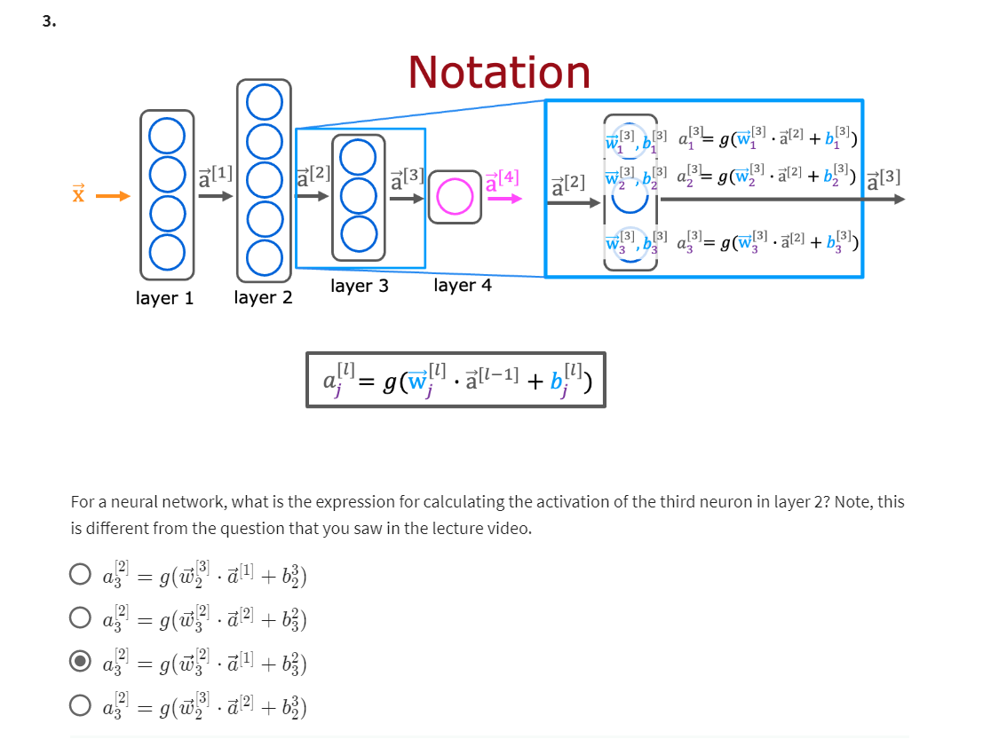
Yes! The superscript [3] refers to layer 3. The subscript 2 refers to the neuron in that layer. The input to layer 2 is the activation vector from layer 1.

[05] TensorFlow implementation

Inference in Code

TensorFlow: One of the leading framework

TensorFlow is one of the leading frameworks to implementing deep
learning algorithms.

When I’m building projects, TensorFlow is actually a tool
that I use the most often. The other popular
tool is PyTorch.

But we’re going to focus in this specialization
on TensorFlow.

In this video, let’s take a
look at how you can implement inferencing code using
TensorFlow. Let’s dive in.

One of the remarkable things
about neural networks is the same algorithm
can be applied to so many different
applications.

For this video and in
some of the labs for you to see what the neural
network is doing, I’m going to use another example
to illustrate inference.

Coffee roasting

Sometimes I do like to roast
coffee beans myself at home. My favorite is actually
Colombian coffee beans.

Can the learning
algorithm help optimize the quality of the beans you get from a roasting
process like this?

When you’re roasting coffee, two parameters you
get to control are the temperature at
which you’re heating up the raw coffee beans to turn them into nicely
roasted coffee beans, as well as the duration or how long are you going
to roast the beans.

In this slightly
simplified example, we’ve created the datasets of different temperatures
and different durations, as well as labels
showing whether the coffee you roasted
is good-tasting coffee.

Where cross here, the positive cross y equals 1
corresponds to good coffee, and all the negative cross
corresponds to bad coffee.

It looks like a reasonable
way to think of this dataset is if you cook
it at too lower temperature, it doesn’t get roasted and
it ends up undercooked.

If you cook it, not
for long enough, the duration is too short, it’s also not a nicely
roasted set of beans.

Finally, if you were to cook it either for too long or for
too higher temperature, then you end up with
overcooked beans. They’re a little
bit burnt beans. There’s not good coffee either. It’s only points within this little triangle here that corresponds to good coffee.

This example is simplified a bit from actual coffee roasting.

Even though this example is a simplified one for the
purpose of illustration, there have actually
been serious projects using machine learning to optimize coffee
roasting as well.

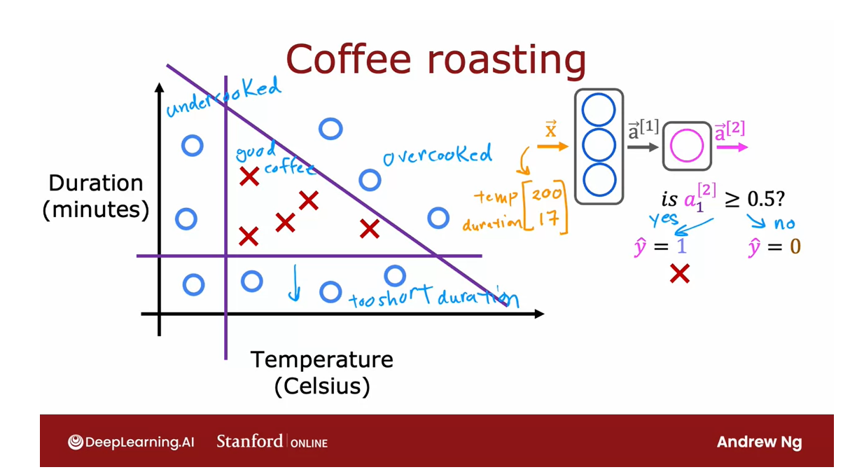
The task is given a feature vector x with both
temperature and duration, say 200 degrees Celsius
for 17 minutes, how can we do inference in a neural network to
get it to tell us whether or not this temperature
and duration setting will result in good
coffee or not? It looks like this.

We’re going to set x to be
an array of two numbers. The input features 200 degrees
celsius and 17 minutes. This here, Layer 1 equals dense
units 3 activation equals sigmoid creates a hidden layer of neurons with
three hidden units, and using as the
activation function, the sigmoid function, and dense here is just
the name of this layer.

Then finally, to compute
the activation values a1, you would write
a1 equals Layer 1 applied to the input features x.

Then you create Layer 1 as this first hidden
layer, the neural network, as dense open
parenthesis units 3, that means three units
or three hidden units in this layer using as the activation function,
the sigmoid function.

Dense is another name for the layers of a neural network that we’ve learned about so far. As you learn more
about neural networks, you learn about other
types of layers as well.

But for now, we’ll just
use the dense layer, which is the layer type
you’ve learned about in the last few videos for
all of our examples.

Next, you compute a1
by taking Layer 1, which is actually a function, and applying this function
Layer 1 to the values of x.

That’s how you get a1, which is going to be a
list of three numbers because Layer 1 had three units. So a1 here may, just for the sake
of illustration, be 0.2, 0.7, 0.3.

Next, for the second
hidden layer, Layer 2, would be dense. Now this time it
has one unit and again to sigmoid
activation function, and you can then
compute a2 by applying this Layer 2 function to the activation values
from Layer 1 to a1. That will give you
the value of a2, which for the sake of
illustration is maybe 0.8.

Finally, if you wish to
threshold it at 0.5, then you can just test if a2 is greater and equal to 0.5 and set y-hat equals to one or zero positive or
negative cross accordingly.

That’s how you do inference in the neural network
using TensorFlow.

There are some
additional details that I didn’t go over here, such as how to load the TensorFlow library
and how to also load the parameters w and
b of the neural network.

But we’ll go over
that in the lab. Please be sure to take
a look at the lab. But these are the key
steps for propagation in how you compute a1 and a2
and optionally threshold a2.

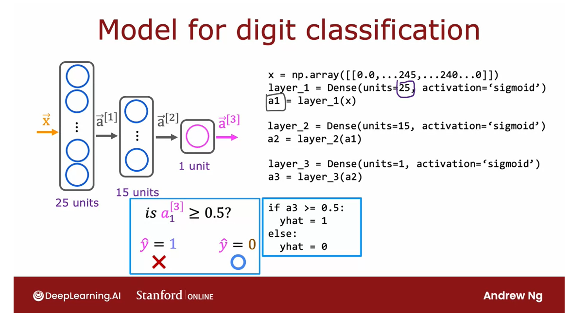
Let’s look at one more example and we’re going to go back to the handwritten digit
classification problem.

In this example, x is a list of the pixel
intensity values. So x is equal to a numpy array of this list
of pixel intensity values.

Then to initialize and carry out one step of
forward propagation, Layer 1 is a dense layer with 25 units and the
sigmoid activation function. You then compute a1 equals the Layer 1
function applied to x.

To build and carry out inference through the
second layer, similarly, you set up Layer 2 as follows, and then computes a2 as
Layer 2 applied to a1. Then finally, Layer 3 is the
third and final dense layer.

Then finally, you can
optionally threshold a3 to come up with a binary
prediction for y-hat.

That’s the syntax for carrying out interference in TensorFlow. One thing I briefly
alluded to is the structure of
the numpy arrays. TensorFlow treats data in a certain way that is
important to get right.

In the next video, let’s take a look at how
TensorFlow handles data.

Data in TensorFlow

Numpy

In this video, I want to step through with
you how data is represented in NumPy and in TensorFlow.

So that as you’re implementing
new neural networks, you can have a consistent framework to
think about how to represent your data.

One of the unfortunate things about the
way things are done in code today is that many, many years ago NumPy was first
created and became a standard library for linear algebra and Python.

And then much later the Google brain team,
the team that I had started and once led created TensorFlow.

And so unfortunately there are some
inconsistencies between how data is represented in NumPy and in TensorFlow.

So it’s good to be aware of these
conventions so that you can implement correct code and hopefully get things
running in your neural networks.

Let’s start by taking a look at
how TensorFlow represents data.

Why double square bracket?

Let’s see you have a data set like
this from the coffee example. I mentioned that you
would write x as follows. So why do you have this
double square bracket here?

Let’s take a look at how NumPy
stores vectors and matrices.

In case you think matrices and vectors are complicated mathematical
concepts don’t worry about it. We’ll go through a few concrete examples
and you’ll be able to do everything you need to do with matrices and vectors
in order to implement your networks.

Let’s start with an example of a matrix. Here is a matrix with 2 rows and
3 columns. Notice that there are one, two rows and 1, 2, 3 columns. So we call this a 2 x 3 matrix.

And so the convention is
the dimension of the matrix is written as the number of rolls
by the number of columns.

So in code to store this matrix,
this 2 x 3 matrix, you just write x = np.array
of these numbers like these.

Where you notice that the square
bracket tells you that 1, 2, 3 is the first row of this matrix and
4, 5, 6 is the second row of this matrix.

And then this open square bracket groups
the first and the second row together. So this sets x to be this
to the array of numbers. So matrix is just a 2D array of numbers.

Let’s look at one more example,
here I’ve written out another matrix. How many rows and
how many columns does this have? Well, you can count this as one, two, three, four rows and
it has one, two columns. So this is a number of rows by the number
of columns matrix, so it’s a 4 x 2 matrix. And so to store this in code,
you will write x equals np.array and then this syntax over here to store these
four rows of matrix in the variable x.

So this creates a 2D array
of these eight numbers. Matrices can have different dimensions. You saw an example of an 2 x 3 matrix and
the 4 x 2 matrix. A matrix can also be other
dimensions like 1 x 2 or 2 x 1.

And we’ll see examples of
these on the next slide.

So what we did previously when
setting x to be input feature vectors, was set x to be equal to np.array
with two square brackets, 200, 17. And what that does is this
creates a 1 x 2 matrix, that is just one row and two columns.

Let’s look at a different example, if you were to define x to be np.array but
now written like this, this creates a 2 x 1 matrix that
has two rows and one column. Because the first row is
just the number 200 and the second row, is just the number 17. And so this has the same numbers but
in a 2 x 1 instead of a 1 x 2 matrix. Enough this example on top
is also called a row vector, is a vector that is just a single row. And this example is also called a column vector because this vector
that just has a single column.

Double square bracket vs. Single square bracket

2D matrix, 1D array (list of numbers, no rows and no columns )

And the difference between using
double square brackets like this versus a single square bracket like this,
is that whereas the two examples on top of 2D arrays where one
of the dimensions happens to be 1.

This example results in a 1D vector. So this is just a 1D array
that has no rows or columns, although by convention we may
right x as a column like this.

So on a contrast this with what we had
previously done in the first course, which was to write x like this
with a single square bracket. And that resulted in
what’s called in Python, a 1D vector instead of a 2D matrix.

And this technically is not 1 x 2 or 2 x
1, is just a linear array with no rows or no columns, but
it’s just a list of numbers.

So where is in course one when we’re
working with linear regression and logistic regression, we use these 1D
vectors to represent the input features x.

With TensorFlow the convention is to
use matrices to represent the data.

And why is there this
switching conventions?

Well it turns out that TensorFlow was
designed to handle very large datasets and by representing the data in
matrices instead of 1D arrays, it lets TensorFlow be a bit more
computational lee efficient internally.

So going back to our original example for
the first training, example in this dataset with features 200°C in 17
minutes, we were represented like this. And so this is actually a 1 x 2 matrix
that happens to have one row and two columns to store the numbers 217.

And in case this seems like a lot
of details and really complicated conventions, don’t worry about it
all of this will become clearer.

And you get to see the concrete
implementations of the code yourself in the optional labs and
in the practice labs. Going back to the code for
carrying out for propagation or influence in the neural network.

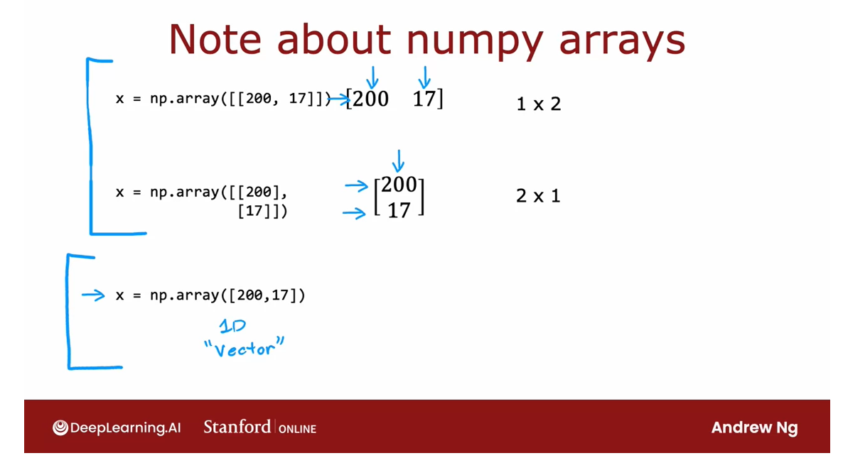
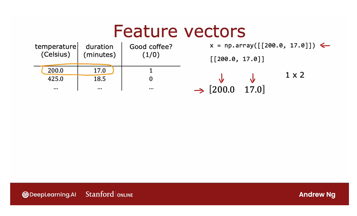
When you compute a1 equals layer
1 applied to x, what is a1? Well, a1 is actually going to
be because the three numbers, is actually going to be a 1 x 3 matrix.

And if you print out a1 you
will get something like this is tf.tensor 0.2, 0.7,
0.3 as a shape of 1 x 3, 1, 3 refers to that
this is a 1 x 3 matrix.

And this is TensorFlow’s way of saying
that this is a floating point number meaning that it’s a number that can
have a decimal point represented using 32 bits of memory in your computer,
that’s where the float 32 is.

What is tensor?

The TensorFlow way to represent data

And what is the tensor? A tensor here is a data type that the
TensorFlow team had created in order to store and carry out computations
on matrices efficiently.

So whenever you see tensor just think
of that matrix on these few slides. Technically a tensor is a little bit
more general than the matrix but for the purposes of this course, think of tensor as just a way
of representing matrices.

So remember I said at the start of this
video that there’s the TensorFlow way of representing the matrix and
the NumPy way of representing matrix.

This is an artifact of
the history of how NumPy and TensorFlow were created and
unfortunately there are two ways of representing a matrix that have
been baked into these systems.

And in fact if you want to
take a1 which is a tensor and want to convert it back to NumPy array,
you can do so with this function a1.numpy.

And it will take the same data and
return it in the form of a NumPy array rather than in the form of a TensorFlow
array or TensorFlow matrix.

Now let’s take a look at what the
activations output the second layer would look like.

Here’s the code that we had from before, layer 2 is a dense layer with one unit and
sigmoid activation and a2 is computed by taking layer 2 and
applying it to a1 so what is a2?

A2, maybe a number like 0.8 and technically this is a 1 x 1 matrix
is a 2D array with one row and one column and so
it’s equal to this number 0.8.

And if you print out a2,
you see that it is a TensorFlow tensor with just one element one
number 0.8 and it is a 1 x 1 matrix. And again it is a float32, decimal points number taking
up 32 bits in computer memory.

Once again you can convert
from a tensorflow tensor to a NumPy matrix using a2.numpy and that will turn this back into
a NumPy array that looks like this.

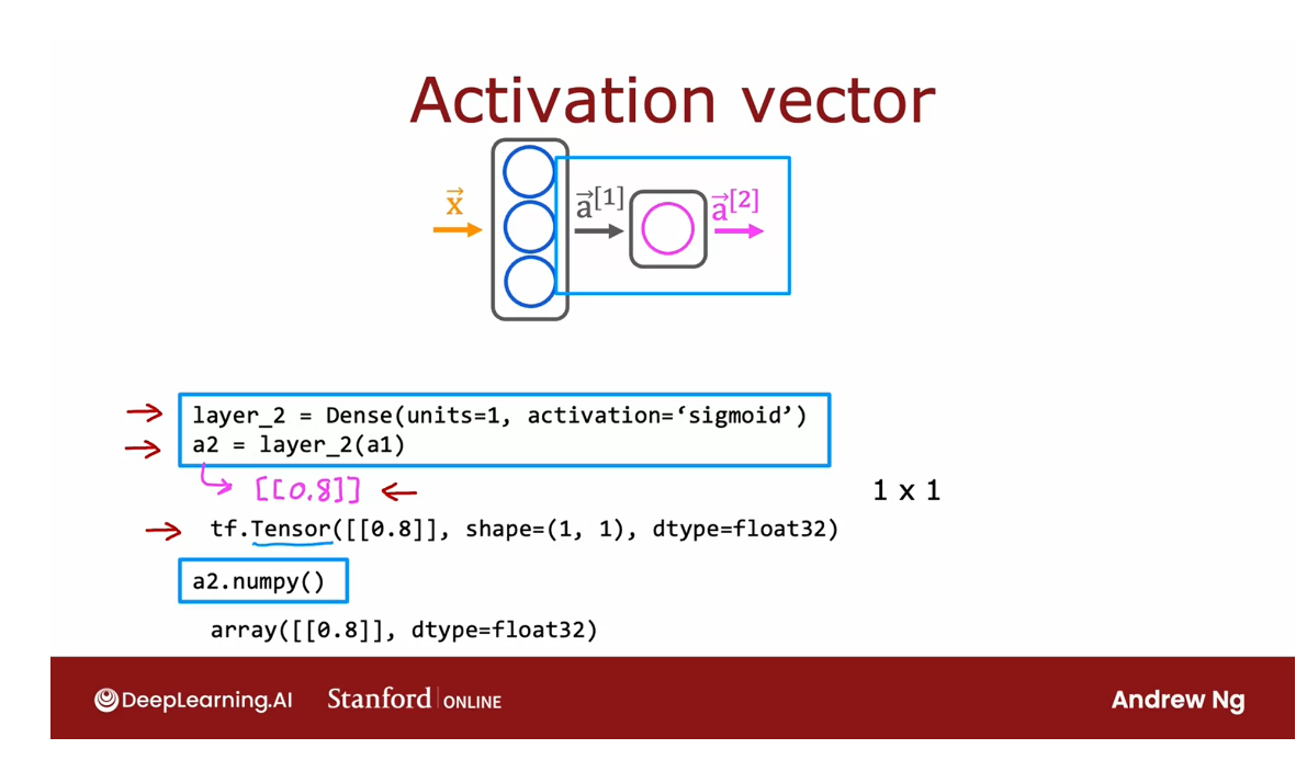
So that hopefully gives you a sense of
how data is represented in TensorFlow and in NumPy. I’m used to loading data and manipulating
data in NumPy, but when you pass a NumPy array into TensorFlow, TensorFlow likes
to convert it to its own internal format.

The tensor and
then operate efficiently using tensors. And when you read the data back
out you can keep it as a tensor or convert it back to a NumPy array.

I think it’s a bit unfortunate that the
history of how these library evolved has let us have to do this
extra conversion work when actually the two libraries
can work quite well together.

But when you convert back and forth,
whether you’re using a NumPy array or a tensor, it’s just something to be
aware of when you’re writing code.

Next let’s take what we’ve learned and put it together to actually
build a neural network. Let’s go see that in the next video.

Building a neural network

So you’ve seen a bunch of tensor flow code
by now learned about how to build a layer in tensor flow, how to do forward prop
through a single layer in tensor flow.

And also learned about
data intensive flow. Let’s put it all together and talk about how to build a neural
network intensive loads.

This is also the last video
on tensor flow for this week. And in this video you also learn about
a different way of building a neural network, that will be even a little bit
simpler than what you’ve seen so far.

So let’s dive in what
you saw previously was. If you want to do for prop,
you initialize the data X create layer one then compute a one,
then create layer two and compute a two.

So this was an explicit way
of carrying out forward problem one layer of
computation at the time. It turns out that tensor
flow has a different way of implementing forward
prop as well as learning.

Let me show you a different way of
building a neural network intensive globe, which is that same as before you’re going
to create layer one and create layer two.

But now instead of you manually taking
the data and passing it to layer one and then taking the activations from
layer one and possibly layer two.

We can instead tell tensorflow that
we would like it to take layer one and layer two and string them together
to form a neural network. That’s what the sequential function
intensive flow does which is it says, the intensive flow please
create a neural network for me by sequentially string together
these two layers that I just created.

It turns out that with
the sequential framework tensorflow can do a lot of work for you.

Let’s say you have a training
set like this on the left.

This is for the coffee example. You can then take the training
data as inputs X and put them into a NP array. This here is a four by two matrix and
the target labels. Y can then be written as follows. And this is just a four dimensional array. Y this set of targets can then
be stored as a one T array like this 1001 corresponding
to four train examples.

And it turns out that given the data,
X and Y stored in this matrix X and
this array, Y. If you want to train this neural network,
all you need to do is call to functions you need to call model
dot compile with some parameters.

We’ll talk more about this next week,
so don’t worry about it for now. And then you need to
call model dot fit X Y, which tells tensor flow to
take this neural network that are created by sequentially
string together layers one and two, and to train it on the data, X and Y. But we’ll learn how but we’ll learn the
details of how to do this next week and then finally how do you do
influence on this neural network?

How do you do forward prop if you
have a new example, say X new, which is NP array with these two
features than to carry out forward prop instead of having to do it
one layer at a time yourself, you just have to call
model predict on X new and this will output the corresponding
value of a two for you given this input value of X.

So model predicts carries out for
propagation and carries an influence for you, using this new network that you
compiled using the sequential function.

Now I want to take these three
lines of code on top and just simplify it a little bit further,
which is when coding intensive flow.

By convention we don’t explicitly
assign the two layers to two variables, layer one and layer two as follows.

But by convention I would usually
just write a code like this, when we say the model is a sequential
model of a few layers strung together.

Sequentially where the first layer one
is a dense layer with three units and activation of sigmoid and
the second layer, is a dense layer with one unit and
again a sigmoid activation function.

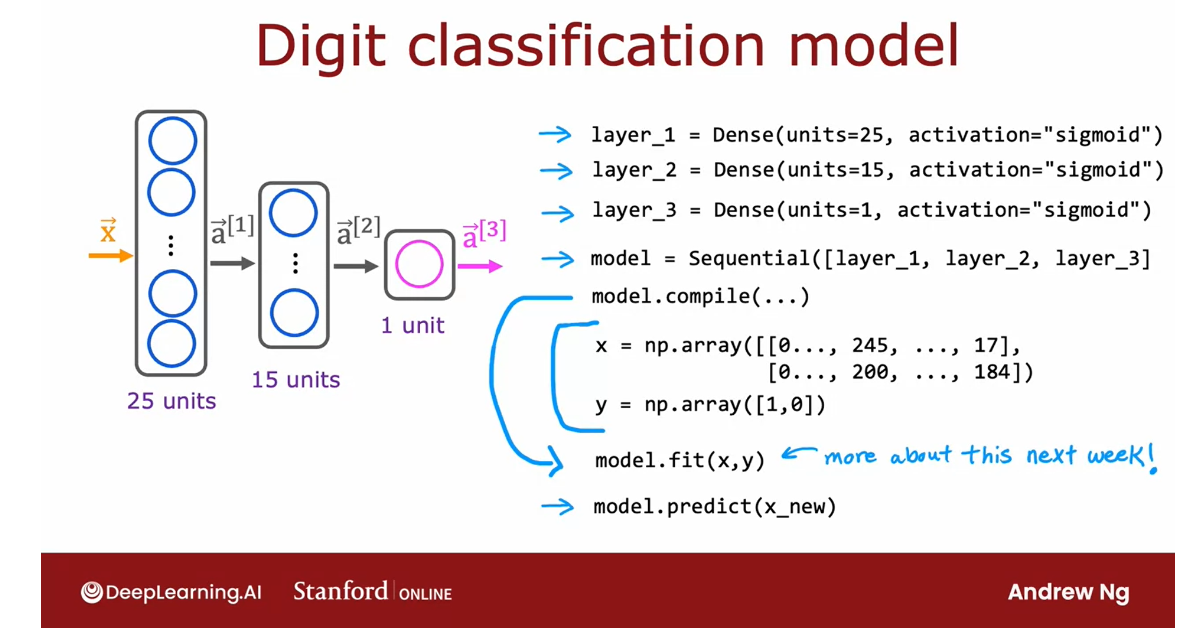
So if you look at others tensor flow code, you often see it look more like
this rather than having an explicit assignment to these layer one and
layer two variables. And so that’s it.

This is pretty much the code you
need in order to train as well as to influence on a neural
network intensive flow. Where again we’ll talk more about
the training bits of this two combined the compiler and
the fit function next week.

Digit classification

Let’s redo this for
the digit classification example as well.

So previously we had X, in this input
layer one is a layer a one equals. They want to apply to X and
so on through layer two and layer three in order to
try to classify a digit, with this new coding convention with
using tensor flow sequential function, you can instead specify what
are layer one, layer two, layer three and tell tensor flow
to string the layers together for you into a new network and same as before.

You can then store
the data in the matrix and run the compile function and
fit the model as follows. Again, more on this next week.

Finally to do inference or to make
predictions you can use model predict on X new and similar to what you saw before
with the coffee classification network by convention, instead of assigning
layer one, layer two, layer three, explicitly like this, we would more
commonly just take these layers and put them directly into
the sequential function.

So you end up with this more compact
code which just tell tensor flow, create a model for me that sequentially
strings together these three layers and then the rest of the code
works the same as before.

So that’s how you have built
a neural network intensive flow.

Now I know that when you’re learning about
these techniques, sometimes someone may ask you to implement these five lines of
code and then you type five lines of code and then someone says congratulations
with just five lines of code.

You built this crazy complicated state of
the art neural network and sometimes that makes you wonder, what exactly did I
do with just these five lines of codes?

One thing I want you to take away from
the machine learning specialization is the ability to use cutting edge
libraries like tensor flow to do your work efficiently.

But I don’t really want you to
just call five lines of code and not really also know what the code is
actually doing underneath the hood.

So in the next video
I’ll let you go back and share with you how you can
implement from scratch by yourself.

For propagation in python, so that you
can understand the whole thing for yourself in practice.

Most machine learning engineers
don’t actually implement for a problem in python that often we just use
libraries like tensor flow and python, but because I want you to understand how
these algorithms work yourself so that if something goes wrong,
you can think through for yourself, what you might need to change was
likely to work was less likely to work.

Let’s also go through what it would
take for you to implement for propagation from scratch because that way,
even when you’re calling a library and having it run efficiently and
do great things in your application, I want you in the back of your mind to
also have that deeper understanding of what your code is actually doing, so
that let’s go on to the next video.

Lab: Coffee Roasting in Tensorflow

Implementing a neural network in tensorflow

Optional Lab - Simple Neural Network

In this lab we will build a small neural network using Tensorflow.

import numpy as np
import matplotlib.pyplot as plt
plt.style.use('./deeplearning.mplstyle')
import tensorflow as tf
from tensorflow.keras.models import Sequential
from tensorflow.keras.layers import Dense
from lab_utils_common import dlc
from lab_coffee_utils import load_coffee_data, plt_roast, plt_prob, plt_layer, plt_network, plt_output_unit
import logging
logging.getLogger("tensorflow").setLevel(logging.ERROR)
tf.autograph.set_verbosity(0)

Dataset

X,Y = load_coffee_data();
print(X.shape, Y.shape)

Output

(200, 2) (200, 1)

Let’s plot the coffee roasting data below. The two features are Temperature in Celsius and Duration in minutes. Coffee Roasting at Home suggests that the duration is best kept between 12 and 15 minutes while the temp should be between 175 and 260 degrees Celsius. Of course, as temperature rises, the duration should shrink.

plt_roast(X,Y)

Output

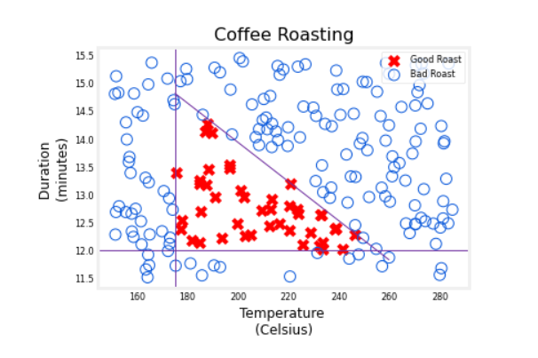
Normalize Data

Fitting the weights to the data (back-propagation, covered in next week’s lectures) will proceed more quickly if the data is normalized. This is the same procedure you used in Course 1 where features in the data are each normalized to have a similar range.
The procedure below uses a Keras normalization layer. It has the following steps:

• create a “Normalization Layer”. Note, as applied here, this is not a layer in your model.
• ‘adapt’ the data. This learns the mean and variance of the data set and saves the values internally.
• normalize the data.
  It is important to apply normalization to any future data that utilizes the learned model.

print(f"Temperature Max, Min pre normalization: {np.max(X[:,0]):0.2f}, {np.min(X[:,0]):0.2f}")
print(f"Duration    Max, Min pre normalization: {np.max(X[:,1]):0.2f}, {np.min(X[:,1]):0.2f}")
norm_l = tf.keras.layers.Normalization(axis=-1)
norm_l.adapt(X)  # learns mean, variance
Xn = norm_l(X)
print(f"Temperature Max, Min post normalization: {np.max(Xn[:,0]):0.2f}, {np.min(Xn[:,0]):0.2f}")
print(f"Duration    Max, Min post normalization: {np.max(Xn[:,1]):0.2f}, {np.min(Xn[:,1]):0.2f}")

Output

Temperature Max, Min pre normalization: 284.99, 151.32
Duration    Max, Min pre normalization: 15.45, 11.51
Temperature Max, Min post normalization: 1.66, -1.69
Duration    Max, Min post normalization: 1.79, -1.70

Tile/copy our data to increase the training set size and reduce the number of training epochs.

Xt = np.tile(Xn,(1000,1))
Yt= np.tile(Y,(1000,1))   
print(Xt.shape, Yt.shape) 

Output

(200000, 2) (200000, 1)

Model

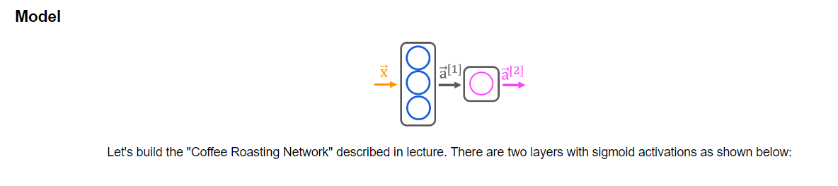
tf.random.set_seed(1234)  # applied to achieve consistent results
model = Sequential(
    [
        tf.keras.Input(shape=(2,)),
        Dense(3, activation='sigmoid', name = 'layer1'),
        Dense(1, activation='sigmoid', name = 'layer2')
     ]
)

Note 1: The tf.keras.Input(shape=(2,)), specifies the expected shape of the input. This allows Tensorflow to size the weights and bias parameters at this point. This is useful when exploring Tensorflow models. This statement can be omitted in practice and Tensorflow will size the network parameters when the input data is specified in the model.fit statement.
Note 2: Including the sigmoid activation in the final layer is not considered best practice. It would instead be accounted for in the loss which improves numerical stability. This will be described in more detail in a later lab.

The model.summary() provides a description of the network:

Model: "sequential"
_________________________________________________________________
 Layer (type)                Output Shape              Param #   
=================================================================
 layer1 (Dense)              (None, 3)                 9         
                                                                 
 layer2 (Dense)              (None, 1)                 4         
                                                                 
=================================================================
Total params: 13
Trainable params: 13
Non-trainable params: 0

The parameter counts shown in the summary correspond to the number of elements in the weight and bias arrays as shown below.

L1_num_params = 2 * 3 + 3   # W1 parameters  + b1 parameters
L2_num_params = 3 * 1 + 1   # W2 parameters  + b2 parameters
print("L1 params = ", L1_num_params, ", L2 params = ", L2_num_params  )

Output

L1 params =  9 , L2 params =  4

Let’s examine the weights and biases Tensorflow has instantiated. The weights $W$ should be of size (number of features in input, number of units in the layer) while the bias $b$ size should match the number of units in the layer:

• In the first layer with 3 units, we expect W to have a size of (2,3) and $b$ should have 3 elements.
• In the second layer with 1 unit, we expect W to have a size of (3,1) and $b$ should have 1 element.

W1, b1 = model.get_layer("layer1").get_weights()
W2, b2 = model.get_layer("layer2").get_weights()
print(f"W1{W1.shape}:\n", W1, f"\nb1{b1.shape}:", b1)
print(f"W2{W2.shape}:\n", W2, f"\nb2{b2.shape}:", b2)

Output

W1(2, 3):
 [[ 0.08 -0.3   0.18]
 [-0.56 -0.15  0.89]] 
b1(3,): [0. 0. 0.]
W2(3, 1):
 [[-0.43]
 [-0.88]
 [ 0.36]] 
b2(1,): [0.]

The following statements will be described in detail in Week2. For now:

• The model.compile statement defines a loss function and specifies a compile optimization.
• The model.fit statement runs gradient descent and fits the weights to the data.

model.compile(
    loss = tf.keras.losses.BinaryCrossentropy(),
    optimizer = tf.keras.optimizers.Adam(learning_rate=0.01),
)

model.fit(
    Xt,Yt,            
    epochs=10,
)

Output

Epoch 1/10
6250/6250 [==============================] - 5s 762us/step - loss: 0.1782
Epoch 2/10
6250/6250 [==============================] - 5s 750us/step - loss: 0.1165
Epoch 3/10
6250/6250 [==============================] - 5s 770us/step - loss: 0.0426
Epoch 4/10
6250/6250 [==============================] - 5s 756us/step - loss: 0.0160
Epoch 5/10
6250/6250 [==============================] - 5s 763us/step - loss: 0.0104
Epoch 6/10
6250/6250 [==============================] - 5s 765us/step - loss: 0.0073
Epoch 7/10
6250/6250 [==============================] - 5s 787us/step - loss: 0.0052
Epoch 8/10
6250/6250 [==============================] - 5s 768us/step - loss: 0.0037
Epoch 9/10
6250/6250 [==============================] - 5s 768us/step - loss: 0.0027
Epoch 10/10
6250/6250 [==============================] - 5s 763us/step - loss: 0.0020
<keras.callbacks.History at 0x7f692802d750>

Updated Weights

After fitting, the weights have been updated:

W1, b1 = model.get_layer("layer1").get_weights()
W2, b2 = model.get_layer("layer2").get_weights()
print("W1:\n", W1, "\nb1:", b1)
print("W2:\n", W2, "\nb2:", b2)

Output

W1:
 [[ -0.21  16.48 -12.21]
 [ -9.5   13.67  -0.28]] 
b1: [-11.73   2.31 -13.14]
W2:
 [[-76.22]
 [-66.  ]
 [-80.35]] 
b2: [45.52]

Next, we will load some saved weights from a previous training run. This is so that this notebook remains robust to changes in Tensorflow over time. Different training runs can produce somewhat different results and the discussion below applies to a particular solution. Feel free to re-run the notebook with this cell commented out to see the difference.

W1 = np.array([
    [-8.94,  0.29, 12.89],
    [-0.17, -7.34, 10.79]] )
b1 = np.array([-9.87, -9.28,  1.01])
W2 = np.array([
    [-31.38],
    [-27.86],
    [-32.79]])
b2 = np.array([15.54])
model.get_layer("layer1").set_weights([W1,b1])
model.get_layer("layer2").set_weights([W2,b2])

Predictions

Once you have a trained model, you can then use it to make predictions. Recall that the output of our model is a probability. In this case, the probability of a good roast. To make a decision, one must apply the probability to a threshold. In this case, we will use 0.5

Let’s start by creating input data. The model is expecting one or more examples where examples are in the rows of matrix. In this case, we have two features so the matrix will be (m,2) where m is the number of examples.
Recall, we have normalized the input features so we must normalize our test data as well.
To make a prediction, you apply the predict method.

X_test = np.array([
    [200,13.9],  # postive example
    [200,17]])   # negative example
X_testn = norm_l(X_test)
predictions = model.predict(X_testn)
print("predictions = \n", predictions)

Output

predictions = 
 [[9.63e-01]
 [3.03e-08]]

Epochs and batches

In the compile statement above, the number of epochs was set to 10. This specifies that the entire data set should be applied during training 10 times. During training, you see output describing the progress of training that looks like this:

Epoch 1/10
6250/6250 [==============================] - 6s 910us/step - loss: 0.1782

The first line, Epoch 1/10, describes which epoch the model is currently running. For efficiency, the training data set is broken into ‘batches’. The default size of a batch in Tensorflow is 32. There are 200000 examples in our expanded data set or 6250 batches. The notation on the 2nd line 6250/6250 [==== is describing which batch has been executed.

To convert the probabilities to a decision, we apply a threshold:

yhat = np.zeros_like(predictions)
for i in range(len(predictions)):
    if predictions[i] >= 0.5:
        yhat[i] = 1
    else:
        yhat[i] = 0
print(f"decisions = \n{yhat}")

Output

decisions = 
[[1.]
 [0.]]

This can be accomplished more succinctly:

yhat = (predictions >= 0.5).astype(int)
print(f"decisions = \n{yhat}")

Output

decisions = 
[[1]
 [0]]

Layer Functions

Let’s examine the functions of the units to determine their role in the coffee roasting decision. We will plot the output of each node for all values of the inputs (duration,temp). Each unit is a logistic function whose output can range from zero to one. The shading in the graph represents the output value.

Note: In labs we typically number things starting at zero while the lectures may start with 1.

plt_layer(X,Y.reshape(-1,),W1,b1,norm_l)

Output

The shading shows that each unit is responsible for a different “bad roast” region. unit 0 has larger values when the temperature is too low. unit 1 has larger values when the duration is too short and unit 2 has larger values for bad combinations of time/temp. It is worth noting that the network learned these functions on its own through the process of gradient descent. They are very much the same sort of functions a person might choose to make the same decisions.

The function plot of the final layer is a bit more difficult to visualize. It’s inputs are the output of the first layer. We know that the first layer uses sigmoids so their output range is between zero and one. We can create a 3-D plot that calculates the output for all possible combinations of the three inputs. This is shown below. Above, high output values correspond to ‘bad roast’ area’s. Below, the maximum output is in area’s where the three inputs are small values corresponding to ‘good roast’ area’s.

plt_output_unit(W2,b2)

Output

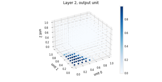
The final graph shows the whole network in action.
The left graph is the raw output of the final layer represented by the blue shading. This is overlaid on the training data represented by the X’s and O’s.
The right graph is the output of the network after a decision threshold. The X’s and O’s here correspond to decisions made by the network.
The following takes a moment to run

netf= lambda x : model.predict(norm_l(x))
plt_network(X,Y,netf)

Output

Congratulations!

You have built a small neural network in Tensorflow.
The network demonstrated the ability of neural networks to handle complex decisions by dividing the decisions between multiple units.

[06] Practice quiz: TensorFlow implementation

Practice quiz: TensorFlow implementation

Latest Submission Grade 100%

Question 2

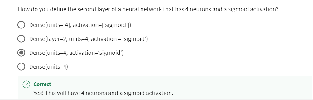
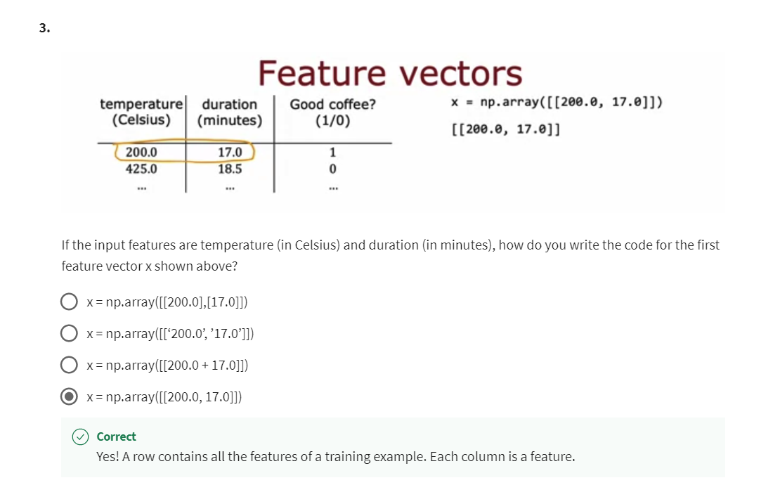
A row contains all the features of a training example. Each column is a feature.

[07] Neural network implementation in Python

Forward prop in a single layer

Implement forward propagation from scratch

if you had to implement forward
propagation yourself from scratch in python, how would you go about doing so,
in addition to gaining intuition about what’s really going on in
libraries like TensorFlow and PyTorch.

If ever some day you decide you
want to build something even better than TensorFlow and PyTorch,
maybe now you have a better idea home, I don’t really recommend doing this for
most people.

But maybe someday, someone will come
up with an even better framework than TensorFlow and PyTorch and whoever does
that may end up having to implement these things from scratch themselves.

Go through quite a bit of code

So let’s take a look, on this slide I’m going to go
through quite a bit of code and you see all this code again later in the
optional lab as was in the practice lab. So don’t worry about having to take
notes on every line of code or memorize every line of code.

You see this code written down in
the Jupyter notebook in the lab and the goal of this video is to just show
you the code to make sure you can understand what it’s doing.

So that when you go to the optional lab
and the practice lab and see the code there, you know what to do so don’t worry
about taking detailed notes on every line. If you can read through the code on this
slide and understand what it’s doing, that’s all you need.

So let’s take a look at how you implement
forward prop in a single layer, we’re going to continue using
the coffee roasting model shown here.

And let’s look at how you would
take an input feature vector x, and implement forward prop
to get this output a2.

In this python implementation, I’m going to use 1D arrays to
represent all of these vectors and parameters, which is why there’s
only a single square bracket here. This is a 1D array in python
rather than a 2D matrix, which is what we had when we
had double square brackets.

Convention: $w_1^{[2]}=w2\_1$

第二层第一个神经元

So the first value you need to compute is, a super strip square bracket 1
subscript 1, which is the first activation value of a1 and
that’s g of this expression over here.

So I’m going to use the convention on
this slide that at a term like w2, 1, I’m going to represent as
a variable w2 and then subscript 1.

This underscore one denotes subscript one,
denotes subscript one so w2 means w superscript 2 in square
brackets and then subscript 1.

So, to compute a1_1,
we have parameters w1_1 and b1_1, which are say 1_2 and -1.

You would then compute
z1_1 as the dot product between that parameter w1_1 and
the input x, and added to b1_1 and
then finally a1_1 is equal to g, the sigmoid function applied to z1_1.

Next let’s go on to compute a1_2,
which again by the convention I described here is going to be a1_2,
written like that.

So similar as what we did on the left, w1_2 is two parameters -3,
4, b1_2 is the term, b 1, 2 over there, so you compute
z as this term in the middle and then apply the sigmoid function and
then you end up with a 1_2, and finally you do the same
thing to compute a1_3.

Output of the first layer: group these three numbers together into an array

Now, you’ve computed these three values,
a1_1, a1_2, and a1_3, and
we like to take these three numbers and group them together into
an array to give you a1 up here, which is the output of the first layer. And so you do that by grouping them
together using a np array as follows, so now you’ve computed a_1,
let’s implement the second layer as well.

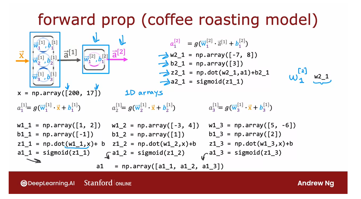
Implement the second layer

So you compute, the output a2,
so a2 is computed using this expression and so
we would have parameters w2_1 and b2_1 corresponding to these parameters.

And then you would compute z as
the dot product between w2_1 and a1, and add b2_1 and then apply
the sigmoid function to get a2_1 and that’s it, that’s how you implement
forward prop using just python and np.

Now, there are a lot of expressions in
this page of code that you just saw, let’s in the next video look at how
you can simplify this to implement forward prop for a more general neural
network, rather than hard coding it for every single neuron like we just did. So let’s go see that in the next video.

General implementation of forward propagation

In the last video,
you saw how to implement forward
prop in Python, but by hard coding lines of
code for every single neuron.

Let’s now take a look at the more general implementation of forward prop in Python. Similar to the previous video, my goal in this video is to
show you the code so that when you see it again
in their practice lab, in the optional labs, you
know how to interpret it.

As we walk through this example, don’t worry about taking notes on every
single line of code.

Just read through the code and understand it

If you can read
through the code and understand it, that’s
definitely enough.

What you can do is write a function to implement
a dense layer, that is a single layer
of a neural network.

I’m going to define
the dense function, which takes as input the activation from
the previous layer, as well as the parameters w and b for the neurons
in a given layer.

Using the example from
the previous video, if layer 1 has three neurons, and if w_1 and w_2
and w_3 are these, then what we’ll do is stack all of these wave
vectors into a matrix.

W matrix: each column represents $w_i$

This is going to be a
two by three matrix, where the first column is the parameter w_1,1
the second column is the parameter w_1, 2, and the third column
is the parameter w_1,3.

Then in a similar way, if you have parameters be, b_1,1 equals negative one, b_1,2 equals one, and so on, then we’re going to stack
these three numbers into a 1D array b as follows, negative one, one, two.

What the dense function
will do is take as inputs the activation
from the previous layer, and a here could be a_0, which is equal to x, or the activation
from a later layer, as well as the w parameters
stacked in columns, like shown on the right, as well as the b parameters also stacked into a 1D array, like shown to the
left over there.

What this function
would do is input a to activation from the
previous layer and will output the activations
from the current layer.

Step through the code of the dense function

Let’s step through the
code for doing this. Here’s the code.

First,
units equals W.shape 1.

W here is a two-by-three matrix, and so the number of
columns is three. That’s equal to the number
of units in this layer. Here, units would
be equal to three.

Looking at the shape of w, is just a way of pulling
out the number of hidden units or the number
of units in this layer.

Next, we set a to be an array of zeros with as many elements
as there are units. In this example, we need to output three
activation values, so this just initializes
a to be zero, zero, zero, an array
of three zeros.

Next, we go through a for
loop to compute the first, second, and third elements of a. For j in range units, so j goes from zero
to units minus one. It goes from 0, 1, 2 indexing from zero
and Python as usual.

This command w equals
W colon comma j, this is how you pull out the jth column of a
matrix in Python.

The first time
through this loop, this will pull the
first column of w, and so will pull out w_1,1. The second time
through this loop, when you’re computing the
activation of the second unit, will pull out the second
column corresponding to w_1, 2, and so on for the third
time through this loop.

Then you compute z using
the usual formula, is a dot product between that parameter w and the activation that
you have received, plus b, j. And then you compute
the activation a, j, equals g sigmoid
function applied to z.

Three times through this
loop and you compute it, the values for all three values of this vector of
activation is a. Then finally you return a.

What does the dense function do?

Inputs the activations from the previous layer, and given the parameters for the current layer, it returns the activations for the next layer.

What the dense
function does is it inputs the activations
from the previous layer, and given the parameters
for the current layer, it returns the activations
for the next layer.

String together a few dense layers sequentially

Given the dense function, here’s how you can string together a few dense
layers sequentially, in order to implement forward
prop in the neural network.

Given the input features x, you can then compute the activations a_1 to be
a_1 equals dense of x, w_1, b_1, where here w_1, b_1 are the parameters, sometimes also
called the weights of the first hidden layer.

Then you can compute a_2
as dense of now a_1, which you just computed above. W_2, b-2 which are
the parameters or weights of this
second hidden layer.

Then compute a_3 and a_4. If this is a neural
network with four layers, then define the output f
of x is just equal to a_4, and so you return f of x.

Notational conventions:

Uppercase or a capital alphabet: matrix

Lowercase: vectors and scalars

Notice that here I’m using W, because under the
notational conventions from linear algebra is
to use uppercase or a capital alphabet is
when it’s referring to a matrix and lowercase refer
to vectors and scalars.

So because it’s a matrix, this is W. That’s it.

You now know how to implement forward prop yourself
from scratch. You get to see all this code
and run it and practice it yourself in the practice lab
coming off to this as well.

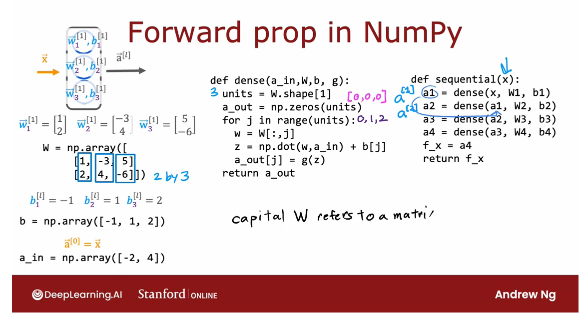
I think that even
when you’re using powerful libraries
like TensorFlow, it’s helpful to know how
it works under the hood.

Because in case
something goes wrong, in case something
runs really slowly, or you have a strange result, or it looks like there’s a bug, your ability to understand
what’s actually going on will make you much
more effective when debugging your code.

When I run machine learning
algorithms a lot of the time, frankly, it doesn’t work. Sophie, not the first time. I find that my ability to debug my code to be a TensorFlow
code or something else, is really important to being an effective machine
learning engineer.

Even when you’re using TensorFlow or some
other framework, I hope that you find this
deeper understanding useful for your own applications
and for debugging your own machine learning
algorithms as well. That’s it. That’s the
last required video of this week with code in it.

In the next video, I’d like to dive
into what I think is a fun and fascinating
topic, which is, what is the relationship
between neural networks and AI or AGI, artificial
general intelligence?

This is a controversial topic, but because it’s been
so widely discussed, I want to share with you
some thoughts on this.

When you are asked, are neural networks at all on the path to human
level intelligence? You have a framework for
thinking about that question. Let’s go take a look
at that fun topic, I think, in the next video.

Lab: CoffeeRoastingNumPy

This lab demonstrates a neural network forwarding path in NumPy.

import numpy as np
import matplotlib.pyplot as plt
plt.style.use('./deeplearning.mplstyle')
import tensorflow as tf
from lab_utils_common import dlc, sigmoid
from lab_coffee_utils import load_coffee_data, plt_roast, plt_prob, plt_layer, plt_network, plt_output_unit
import logging
logging.getLogger("tensorflow").setLevel(logging.ERROR)
tf.autograph.set_verbosity(0)

DataSet

This is the same data set as the previous lab.

X,Y = load_coffee_data();
print(X.shape, Y.shape)

Output

(200, 2) (200, 1)

Let’s plot the coffee roasting data below. The two features are Temperature in Celsius and Duration in minutes. Coffee Roasting at Home suggests that the duration is best kept between 12 and 15 minutes while the temp should be between 175 and 260 degrees Celsius. Of course, as the temperature rises, the duration should shrink.

plt_roast(X,Y)

Output

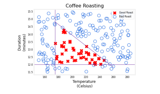
Normalize Data

To match the previous lab, we’ll normalize the data. Refer to that lab for more details

print(f"Temperature Max, Min pre normalization: {np.max(X[:,0]):0.2f}, {np.min(X[:,0]):0.2f}")
print(f"Duration    Max, Min pre normalization: {np.max(X[:,1]):0.2f}, {np.min(X[:,1]):0.2f}")
norm_l = tf.keras.layers.Normalization(axis=-1)
norm_l.adapt(X)  # learns mean, variance
Xn = norm_l(X)
print(f"Temperature Max, Min post normalization: {np.max(Xn[:,0]):0.2f}, {np.min(Xn[:,0]):0.2f}")
print(f"Duration    Max, Min post normalization: {np.max(Xn[:,1]):0.2f}, {np.min(Xn[:,1]):0.2f}")

Output

Temperature Max, Min pre normalization: 284.99, 151.32
Duration    Max, Min pre normalization: 15.45, 11.51
Temperature Max, Min post normalization: 1.66, -1.69
Duration    Max, Min post normalization: 1.79, -1.70

Numpy Model (Forward Prop in NumPy)

Let’s build the “Coffee Roasting Network” described in lecture. There are two layers with sigmoid activations.

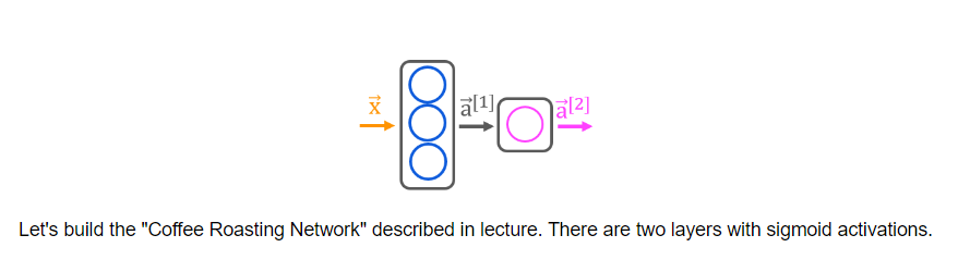
As described in lecture, it is possible to build your own dense layer using NumPy. This can then be utilized to build a multi-layer neural network.

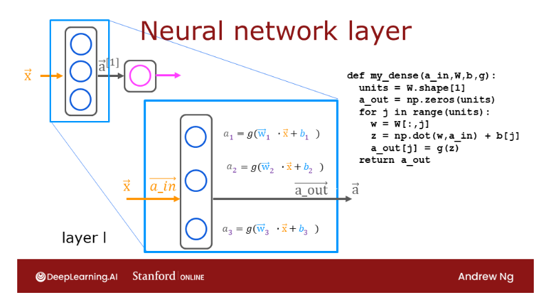
In the first optional lab, you constructed a neuron in NumPy and in Tensorflow and noted their similarity. A layer simply contains multiple neurons/units. As described in lecture, one can utilize a for loop to visit each unit (j) in the layer and perform the dot product of the weights for that unit (W[:,j]) and sum the bias for the unit (b[j]) to form z. An activation function g(z) can then be applied to that result. Let’s try that below to build a “dense layer” subroutine.

def my_dense(a_in, W, b, g):
    """
    Computes dense layer
    Args:
      a_in (ndarray (n, )) : Data, 1 example 
      W    (ndarray (n,j)) : Weight matrix, n features per unit, j units
      b    (ndarray (j, )) : bias vector, j units  
      g    activation function (e.g. sigmoid, relu..)
    Returns
      a_out (ndarray (j,))  : j units|
    """
    units = W.shape[1]
    a_out = np.zeros(units)
    for j in range(units):               
        w = W[:,j]                                    
        z = np.dot(w, a_in) + b[j]         
        a_out[j] = g(z)               
    return(a_out)

这里第一眼不知道W.shape[1] 是干啥的，看功能描述得知， W 是 2D的矩阵，(每个unit的特征数，多少个unit)

The following cell builds a two-layer neural network utilizing the my_dense subroutine above.

两层的神经网络

def my_sequential(x, W1, b1, W2, b2):
    a1 = my_dense(x,  W1, b1, sigmoid)
    a2 = my_dense(a1, W2, b2, sigmoid)
    return(a2)

We can copy trained weights and biases from the previous lab in Tensorflow.

W1_tmp = np.array( [[-8.93,  0.29, 12.9 ], [-0.1,  -7.32, 10.81]] )
b1_tmp = np.array( [-9.82, -9.28,  0.96] )
W2_tmp = np.array( [[-31.18], [-27.59], [-32.56]] )
b2_tmp = np.array( [15.41] )

Predictions

Once you have a trained model, you can then use it to make predictions. Recall that the output of our model is a probability. In this case, the probability of a good roast. To make a decision, one must apply the probability to a threshold. In this case, we will use 0.5

def my_predict(X, W1, b1, W2, b2):
    m = X.shape[0]
    p = np.zeros((m,1))
    for i in range(m):
        p[i,0] = my_sequential(X[i], W1, b1, W2, b2)
    return(p)

We can try this routine on two examples:

X_tst = np.array([
    [200,13.9],  # postive example
    [200,17]])   # negative example
X_tstn = norm_l(X_tst)  # remember to normalize
predictions = my_predict(X_tstn, W1_tmp, b1_tmp, W2_tmp, b2_tmp)

To convert the probabilities to a decision, we apply a threshold:

yhat = np.zeros_like(predictions)
for i in range(len(predictions)):
    if predictions[i] >= 0.5:
        yhat[i] = 1
    else:
        yhat[i] = 0
print(f"decisions = \n{yhat}")

Output

decisions = 
[[1.]
 [0.]]

This can be accomplished more succinctly:

yhat = (predictions >= 0.5).astype(int)
print(f"decisions = \n{yhat}")

Output

decisions = 
[[1]
 [0]]

Network function

This graph shows the operation of the whole network and is identical to the Tensorflow result from the previous lab.
The left graph is the raw output of the final layer represented by the blue shading. This is overlaid on the training data represented by the X’s and O’s.
The right graph is the output of the network after a decision threshold. The X’s and O’s here correspond to decisions made by the network.

netf= lambda x : my_predict(norm_l(x),W1_tmp, b1_tmp, W2_tmp, b2_tmp)
plt_network(X,Y,netf)

Output

Congratulations!

You have built a small neural network in NumPy.
Hopefully this lab revealed the fairly simple and familiar functions which make up a layer in a neural network.

[08] Practice quiz: Neural network implementation in Python

Neural network implementation in Python

Latest Submission Grade 100%

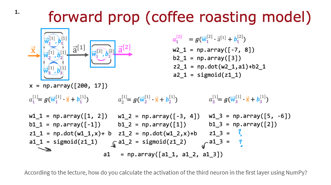
[09] Speculations on artificial general intelligence (AGI)

Is there a path to AGI?

Hold a dream of AI alive

Ever since I was a teenager starting to play around
with neural networks, I just felt that
the dream of maybe someday building an AI system that’s as intelligent as myself or as intelligent
as a typical human, that that was one of the
most inspiring dreams of AI. I still hold that
dream alive today.

But I think that the
path to get there is not clear and could
be very difficult.

I don’t know whether
it would take us mere decades and whether we’ll see breakthroughs
within our lifetimes, or if it may take centuries
or even longer to get there.

Let’s take a look
at what this AGI, artificial general
intelligence dream is like and speculate a bit on what might
be possible paths, unclear paths, difficult
paths to get there someday.

I think there’s been a
lot of unnecessary hype about AGI or artificial
general intelligence.

Maybe one reason for that is AI actually includes two
very different things.

One is ANI which stands for artificial
narrow intelligence.

ANI has made tremendous progress

It’s creating tremendous value in the world today

This is an AI system
that does one thing, a narrow task, sometimes really well and can be
incredibly valuable, such as the smart speaker or self-driving car or web search, or AI applied to specific applications such
as farming or factories.

Over the last several years, ANI has made tremendous
progress and it’s creating, as you know, tremendous
value in the world today.

Because ANI is a subset of AI, the rapid progress in ANI
makes it logically true that AI has also made tremendous
progress in the last decade.

There’s a different idea in AI, which is AGI, artificial
general intelligence. There’s hope of
building AI systems that could do anything
a typical human can do.

Despite all the progress in ANI and therefore
tremendous progress in AI, I’m not sure how much
progress, if any, we’re really making toward AGI. I think all the progress
in ANI has made people conclude correctly that there’s tremendous progress in AI.

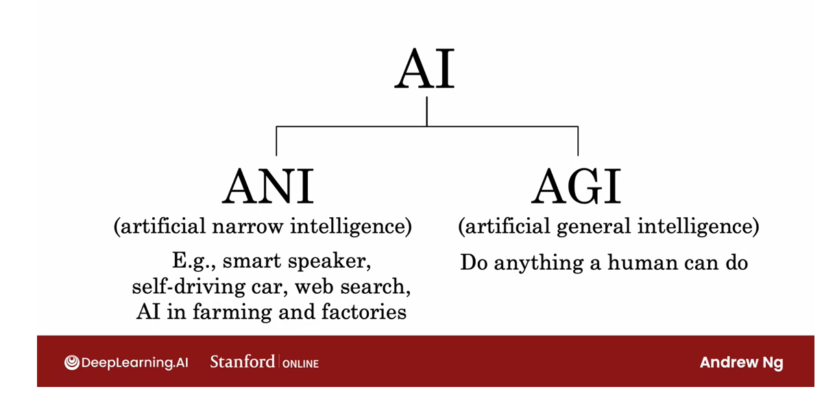
Artificial General Intelligence

AI

• ANI: Artificial Narrow Intelligence

• AGI: Artificial General Intelligence

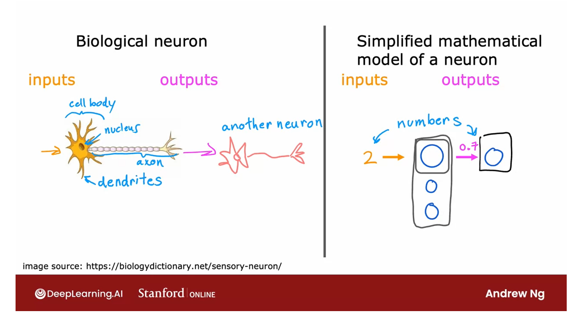
But that has caused some
people to conclude, I think incorrectly that
a lot of progress in AI necessarily means
that there’s a lot of progress towards AGI.

If you have else
about AI and AGI, sometimes you might find drawing this picture useful
for explaining some of the things going on in AI as
well and some of the sources of unnecessary hype about AGI.

With the rise of
modern deep learning, we started to simulate
neurons and with faster and faster computers and even GPUs we can simulate
even more neurons.

I think there was this big hope many years ago that, boy, if only we could simulate a
lot of neurons then we can simulate the human
brain or something like a human brain and we’ve
really intelligent systems.

Simulate the human brain is incredibly difficult.

Sadly, it’s turned out not to be quite as simple as that.

I think two reasons
for this is first, if you look at the artificial neural
networks we’re building, they are so simple that a logistic regression unit
is really nothing like what any biological neuron
is doing is so much simpler than what any neuron in your brain or mine is doing.

Second, even to this day, I think we have almost no
idea how the brain works.

There are still
fundamental questions about how exactly does a neuron map from inputs to outputs that we just
don’t know today.

Trying to simulate
that in a computer, much less a single logistic
function is just so far from an accurate model of what the human brain
actually does.

Given our very limited
understanding both now and probably for the near future of how
the human brain works, I think just trying to
simulate the human brain as a path to AGI will be an
incredibly difficult path.

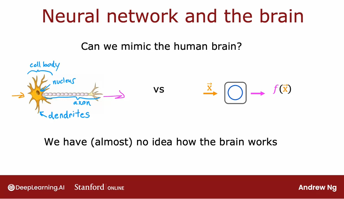
The “One learning algorithm” hypothesis

Having said that, is there any hope of within our lifetimes seeing
breakthroughs in AGI?

Let me share with you
some evidence that helps me keep that hope
alive, at least for myself.

There have been some
fascinating experiments done on animals that shows or strongly suggests that the same piece of biological brain tissue can do a surprisingly wide
range of tasks.

One learning algorithm hypothesis

This has led to the one learning algorithm hypothesis
that maybe a lot of intelligence could be due to one or a small handful
of learning algorithms.

If only we could figure out what that one or small handful
of algorithms are, we may be able to implement
that in a computer someday.

Let me share with you some
details of those experiments. This is a result
due to Roe et al. from many decades ago.

Auditory cortex

The part of your brain shown here is your auditory cortex, and your brain is wired to feed signals from your ears in the form of
electrical impulses, depending on what
sound your ear is detecting to that
auditory cortex.

It turns out that if
you were to rewire an animal brain,s to cut the wire between the ear
and the auditory cortex, and instead feed in images
to the auditory cortex, then the auditory
cortex learns to see.

Auditory refers to sound, and so this piece of the brain that in most people
learns to here, when it is fed different data, it instead learns to see.

Somatosensory cortex: touch processing

Here’s another example. This part of your brain is
your somatosensory cortex, somatosensory refers
to touch processing.

If you were to similarly rewire the brain to cut
the connection from the touch sensors to that
part of the brain and instead rewire the brain
to feed in images, then the somatosensory
cortex learns to see.

There’s been a sequence
of experiments like this, showing that many different
parts of the brain, just depending on what data
is given can learn to see, or learn to feel, or learn to hear as if there was maybe one algorithm that just depending on what
data or this given, learns to process that
inputs accordingly.

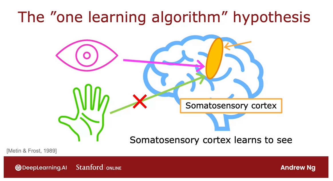
cortex: the outer layer of an organ, especially the brain

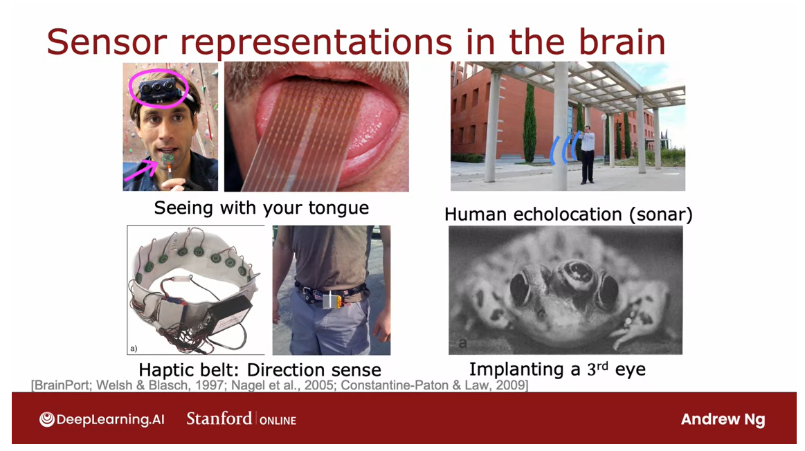
There happens systems built which take a camera
may be mounted to someone’s forehead and
maps it to a pattern of voltages in a grid
on someone’s tongue.

By mapping a grayscale image to a pattern of voltages
on your tongue, this can help people
that are not cited line individuals learn
to see with your tongue, or they’ve been fascinating
experiments with human echolocation
or humans sonar, so animals like dolphins
and bats use sonar to see, and researchers have found that if you train humans
to make clicking sounds, and listen to how that
bounces off surroundings, humans can sometimes learn some degree of
human echolocation.

Or this is a haptic belt, and my research lab
at Stanford once built something like
this before as well, but if you mount a ring of
buzzes around your waist and program it using a
magnetic compass, so that say, the buzzers to the
North most direction are always vibrating slowly, then you somehow gain
a direction sense, which some animals
have, but humans don’t.

Then it just feels like you’re walking around and you
just know where North is, it doesn’t feel like that
part of my waist is buzzing, it feels like, oh, I know
where that north is.

Or surgeries implant a third eye onto frog and the brain just learns with you
with this input.

The human brain is amazingly adaptable

There have been a variety of experiments like
these just showing that the human brain is
amazingly adaptable, neuroscientists say
is amazingly plastic, they just mean adaptable to bewildering range
of sensor inputs, and so the question is, if the same piece of brain
tissue can learn to see, or touch, or feel, or even other things, what is the average of users, and can we replicate
this algorithm and implemented in a computer?

I do feel bad for the
frog and other animals, or which these
experiments were done, although I think the conclusions are also quite fascinating.

Even to this day, I think
working on AGI is one of the most fascinating science and engineering
problems of all time, and maybe you will choose
someday to do research on it.

However, I think it’s important
to avoid over-hyping, I don’t know if the
brain is really one or a small handful
of algorithms, and even if it were, I have no idea, and I don’t think anyone
knows what the algorithm is, but I still this hope alive, and maybe it is, and maybe we could, through a lot of hard work, someday discover an
approximation to it.

I still find this one of the
most fascinating topics, I really think about it in my spare time and maybe someday, you be the one to make a
contribution to this problem.

In the short term, I think
even without pursuing AGI, machine learning
and neural networks are very powerful tool, and even without
trying to go all the way to build
human-level intelligence, I think you find neural networks to be
an incredibly powerful, and useful set of tools for applications that
you might build.

That’s it for the required
videos of this week, congratulations on getting to
this point in the lessons.

After this, we’ll also have a few optional videos
to dive a little bit more deeply into efficient implementations
of neural networks. In particular, in the
optional videos to come, I’d like to share with
you some details of how to vectorize implementations
of neural networks. I hope you also take a
look at those videos.

[10] Vectorization (optional)

How neural networks are implemented efficiently

Scale up NN: NN can be vectorized

One of the reasons that
deep learning researchers have been able to scale
up neural networks, and thought really
large neural networks over the last decade, is because neural networks
can be vectorized.

Parallel computing hardware: very good at doing very large matrix multiplications.

They can be implemented very efficiently using
matrix multiplications.

It turns out that parallel computing
hardware, including GPUs, but also some CPU
functions are very good at doing very large
matrix multiplications.

In this video, we’ll
take a look at how these vectorized implementations
of neural networks work.

Without these ideas, I
don’t think deep learning would be anywhere near a
success and scale today.

For loop implementation

Here on the left is the
code that you had seen previously of how you would
implement forward prop, or forward propagation, in a single layer.

X here is the input, W, the weights of
the first, second, and third neurons, say, parameters B, and then this is the same code as
which we saw before.

This will output three numbers, say, like that. If you actually implement
this computation, you get 1, 0, 1.

Vectorized implementation

It turns out you can develop a vectorized implementation
of this function as follows.

Set X to be equal to this. Notice the double
square brackets. This is now a 2D array,
like in TensorFlow. W is the same as before, and B, I’m now using B, is also a one by three 2D array. Then it turns out that
all of these steps, this for loop inside, can be replaced with just
a couple of lines of code, Z equals np.matmul.

Matmul is how NumPy carries
out matrix multiplication.

Where now X and W
are both matrices, and so you just
multiply them together.

It turns out that this for loop, all of these lines
of code can be replaced with just a
couple of lines of code, which gives a vectorized
implementation of this function.

You compute Z, which is now a matrix again, as numpy.matmul
between A in and W, where here A in and
W are both matrices, and matmul is how NumPy carries out a matrix
multiplication.

It multiplies two
matrices together, and then adds the
matrix B to it. Then A out is equal to the
activation function g, that is the sigmoid function, applied element-wise
to this matrix Z, and then you finally
return A out. This is what the
code looks like.

Notice that in the
vectorized implementation, all of these quantities, x, which is fed into the value
of A in as well as W, B, as well as Z and A out, all of these are now 2D arrays. All of these are matrices.

This turns out to be a very efficient
implementation of one step of forward propagation through a dense layer
in the neural network.

This is code for a vectorized implementation of forward prop in a
neural network.

But what is this code doing and how does
it actually work? What is this matmul
actually doing?

In the next two videos, both also optional, we’ll go over matrix
multiplication and how that works. If you’re familiar
with linear algebra, if you’re familiar with
vectors, matrices, transposes, and matrix multiplications, you can safely just
quickly skim over these two videos and jump to
the last video of this week.

Then in the last video of
this week, also optional, we’ll dive into more
detail to explain how matmul gives you this
vectorized implementation. Let’s go on to the next video, where we’ll take a look at
what matrix multiplication is.

Matrix multiplication

Dot pruducts

You know that a matrix is just a block or 2D
array of numbers.

What does it mean to multiply two matrices? Let’s take a look.

In order to build up to
multiplying matrices, let’s start by looking at how we take dot products
between vectors.

Let’s use the example of taking the dot product
between this vector 1, 2 and this vector 3, 4. If z is the dot product
between these two vectors, then you compute z by multiplying the first element
by the first element here, it’s 1 times 3, plus the second element times the second element
plus 2 times 4, and so that’s just 3 plus 8, which is equal to 11.

In the more general case, if z is the dot product between
a vector a and vector w, then you compute z by multiplying the first
element together and then the second elements
together and the third and so on and then adding up
all of these products.

That’s the vector,
vector dot product.

It turns out there’s another equivalent way of
writing a dot product, which has given a vector a, that is, 1, 2
written as a column. You can turn this into a row.

That is, you can
turn it from what’s called a column vector to a row vector by taking
the transpose of a.

Transpose of a vector: take a column vector and lay its elements on the side

The transpose of the
vector a means you take this vector and lay its
elements on the side like this.

It turns out that if you
multiply a transpose, this is a row vector, or you can think of this as
a one-by-two matrix with w, which you can now think of
as a two-by-one matrix.

Then z equals a transpose times
w and this is the same as taking the dot product
between a and w.

To recap, z equals the dot
product between a and w is the same as z
equals a transpose, that is a laid on the side, multiplied by w and this will be useful for understanding matrix
multiplication.

That these are just
two ways of writing the exact same computation
to arrive at z.

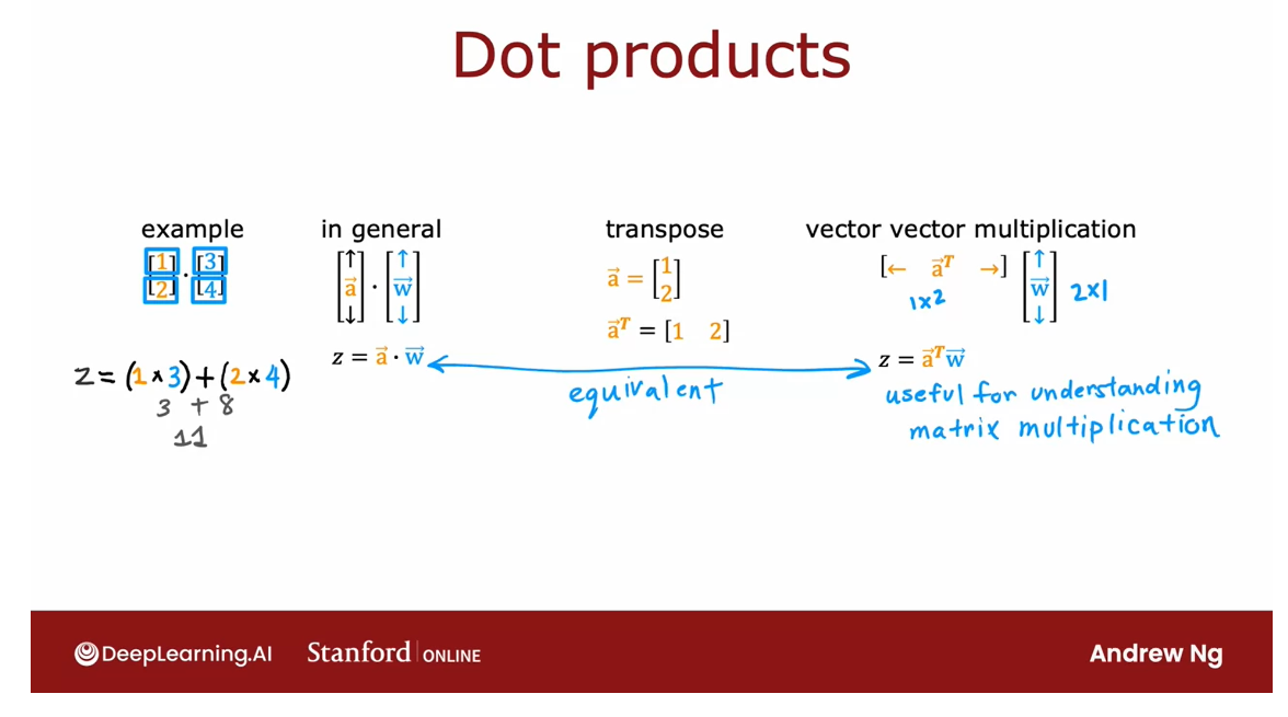
Vector matrix multiplication

Now let’s look at vector
matrix multiplication, which is when you
take a vector and you multiply a vector by a matrix.

Here again is the vector a 1, 2 and a transpose is
a laid on the side, so rather than this
think of this as a two-by-one matrix it
becomes a one-by-two matrix.

Let me now create a two-by-two matrix w
with these four elements, 3, 4, 5, 6. If you want to compute Z as a transpose times w.

Let’s see
how you go about doing so.

It turns out that Z is going
to be a two-by-one matrix, and to compute the
first value of Z we’re going to take a transpose, 1, 2 here, and multiply that
by the first column of w, that’s 3, 4.

To compute the
first element of Z, you end up with 1 times
3 plus 2 times 4, which we saw earlier
is equal to 11, and so the first
element of Z is 11.

Let’s figure out what’s
the second element of Z. It turns out you just
repeat this process, but now multiplying
a transpose by the second column of w.

To do that computation, you have 1 times
5 plus 2 times 6, which is equal to 5
plus 12, which is 17. That’s equal to 17.

Z is equal to this one-by-two
matrix, 11 and 17.

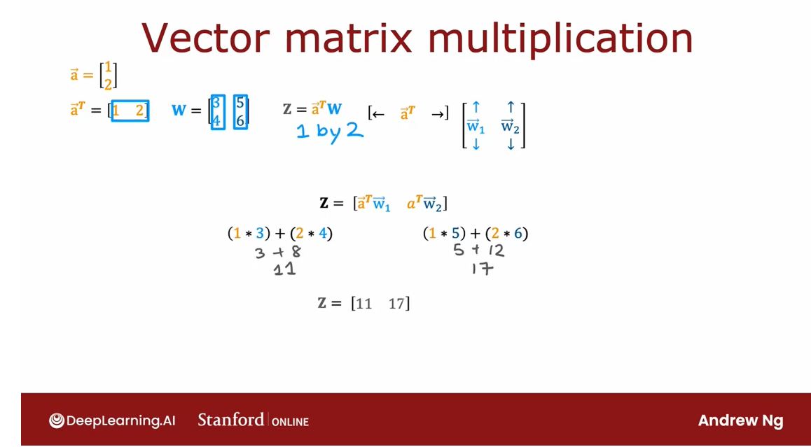
Matrix matrix multiplication

Now, just one last thing, and then that’ll take us
to the end of this video, which is how to take vector matrix multiplication
and generalize it to matrix matrix
multiplication.

I have a matrix A with
these four elements, the first column is 1, 2 and the second
column is negative 1, negative 2 and I want
to know how to compute a transpose times w.

Unlike the previous slide, A now is a matrix rather
than just the vector or the matrix is just a set of different vectors stacked
together in columns.

First let’s figure out
what is A transpose.

How to compute a matrix transpose?

Take the columns and lay them on the side, one column at a time

In order to compute A transpose, we’re going to take
the columns of A and similar to what happened
when you transpose a vector, we’re going to take the columns and lay them on the side, one column at a time.

The first column 1, 2 becomes the first row 1, 2, let’s just laid on side, and this second
column, negative 1, negative 2 becomes laid
on the side negative 1, negative 2 like this.

The way you transpose
a matrix is you take the columns and you just lay
the columns on the side, one column at a time, you end up with this
being A transpose.

Next we have this matrix W, which going to
write as 3,4, 5,6. There’s a column 3, 4
and the column 5, 6.

One way I encourage you
to think of matrices.

At least there’s useful for neural network implementations
is if you see a matrix, think of the columns of the matrix and if you see
the transpose of a matrix, think of the rows of that
matrix as being grouped together as illustrated here, with A and A transpose
as well as W.

Now, let me show you how to
multiply A transpose and W.

In order to carry out this computation let me
call the columns of A, a_1 and a_2 and that
means that a_1 transpose, this the first row
of A transpose, and a_2 transpose is the
second row of A transpose.

Then same as before, let me call the columns
of W to be w_1 and w_2. It turns out that to
compute A transpose W, the first thing we
need to do is let’s just ignore the second row of A and let’s just
pay attention to the first row of A and
let’s take this row 1, 2 that is a_1 transpose
and multiply that with W.

You already know how to do that from
the previous slide. The first element is 1, 2, inner product or dot
product we’ve 3, 4. That ends up with 3 times 1
plus 2 times 4, which is 11. Then the second element is 1, 2 A transpose, inner product we’ve 5, 6. There’s 5 times 1
plus 6 times 2, which is 5 plus 12, which is 17.

That gives you the
first row of Z equals A transpose
W. All we’ve done is take a_1 transpose and multiply that by W. That’s exactly what we did on
the previous slide.

Next, let’s forget a_1 for now, and let’s just look
at a_2 and take a_2 transpose and multiply
that by W. Now we have a_2 transpose times W.

To compute that first we
take negative 1 and negative 2 and dot
product that with 3, 4. That’s negative 1
times 3 plus negative 2 times 4 and that turns
out to be negative 11.

Then we have to compute a_2 transpose times
the second column, and has negative 1 times 5
plus negative 2 times 6, and that turns out
to be negative 17.

You end up with A
transpose times W is equal to this two-by-two
matrix over here.

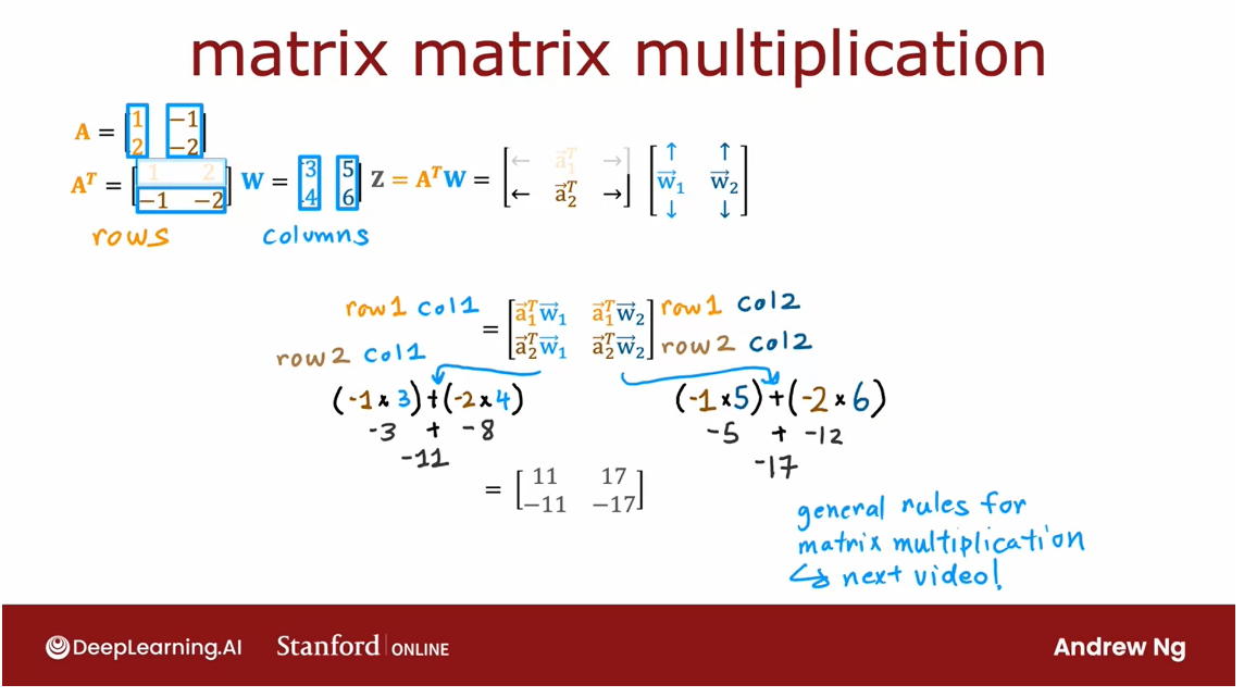
Let’s talk about
the general form of matrix matrix multiplication.

This was an example of how you multiply a vector with a matrix, or a matrix with a matrix is a lot of
dot products between vectors but ordered in a certain way to construct
the elements of the upper Z, one element at a time.

I know this was a lot, but in the next video, let’s look at the
general form of how a matrix matrix
multiplication is defined and I hope that will
make all this clear as well. Let’s go on to the next video.

Matrix multiplication rules

So let’s take a look at the general form
of how you multiply two matrices together.

And then in the last video after this one,
we’ll take this and apply it to the vectorized
implementation of a neural network.

Let’s dive in.

Here’s the matrix A, which is a 2 by 3 matrix because it has two rows and
three columns. As before I encourage you to
think of the columns of this matrix as three vectors,
vectors a1, a2 and a3.

And what we’re going to do
is take A transpose and multiply that with the matrix W.

The first, what is A transpose?

Well, A transpose is obtained by
taking the first column of A and laying it on the side like this and
then taking the second column of A and laying on his side like this.

And then the third column of A and
laying on the side like that. And so these roles are now A1 transpose, A2 transpose and A3 transpose.

Next, here’s the matrix W. I encourage you to think
of W as factors w1, w2, w3, and w4 stacked together.

As so let’s look at how you then
compute A transpose times W. Now, notice that I’ve also used
slightly different shades of orange to denote the different columns of A,
where the same shade corresponds to numbers that we think of as
grouped together into a vector.

And that same shade is used to indicate
different rows of A transpose because the different rows of A transpose are A1
transpose, A2 transpose and A3 transpose.

And in a similar way, I’ve used different shades to
denote the different columns of W. Because the numbers
are the same shade of blue, are the ones that are grouped together to
form the vectors w1, w 2, or w3 or w4.

How to compute A transpose times W

Now, let’s look at how you can
compute A transpose times W.

I’m going to draw vertical bows to
the different shades of blue and horizontal bars with the different
shades of orange to indicate which elements of Z that is
A transpose W are influenced or affected by the different
roles of A transpose and which are influenced or
affected by the different columns of W.

So for example,
let’s look at the first Column of W. So that’s w1 as indicated by
the lightest shade of blue here. So w1 will influence or
will correspond to this first column of Z shown here
by this lighter shade of blue.

And the values of this second
column of W that is w2 as indicated by this second lighter shade of blue
will affect the values computed into second column of Z and so
on for the third and fourth columns.

Correspondingly, let’s
look at A transpose.

A1 transpose is the first row
of A transpose as indicated by the lightest shade of orange and
A1 transpose will effect or influence or correspond to
the values in the first row of Z.

And A2 transpose will influence
the second row of Z and A3 transports will influence or
correspond to this third row of Z.

So let’s figure out how
to compute the matrix Z, which is going to be a 3 by 4 matrix. So with 12 numbers altogether.

Let’s start off and figure out how to
compute the number in the first row, in the first column of Z.

So this upper left most element here
because this is the first row and first column corresponding to the lighter shade
of orange and the lighter shade of blue.

The way you compute that is to grab
the first row of a transpose and the first column of W and
take their inner product or the product.

And so
this number is going to be (1,2) [UNKNOWN ]product with (3,4) which
is (1 * 3) + (2 * 4) = 11.

Let’s look at the second example. How would you compute this element of Z.

So this is in the third row,
row 1, row 2, row 3. So this is in row 3 and
the second column, column 1, column 2. So to compute the number in row 3,
column 2 of Z, you would now grab row
3 of A transpose and column 2 of W and
dot product those together.

Notice that this corresponds to
the darkest shade of orange and the second lightest shade of blue. And to compute this,
this is (0.1 * 5) +(0.2 * 6), which is (0.5 + 1.2),
which is equal to 1.7. So to compute the number in row 3,
column 2 of Z, you grab the third row,
row 3 of a transpose and column 2 of W.

Let’s look at one more example and
let’s see if you can figure this one out. This is row 2, column 3 of the matrix Z. Why don’t you take a look and
see if you can figure out which row and which column to grab the dot
product together and therefore what is the number that will
go in this element of this matrix.

Hopefully you got that.

You should be grabbing row 2 of
A transpose and column 3 of W. And when you dot product
that together you have A2 transpose w3 is (-1 * 7) + (-2 * 8 ), which is (-7 + -16),
which is equal to -23.

And so that’s how you compute
this element of the matrix Z.

And it turns out if you do this for every
element of the matrix Z, then you can compute all of the numbers in this matrix
which turns out to look like that.

Feel free to pause the video if you want
and picking the elements and double check that the formula we’ve been going
through gives you the right value for Z.

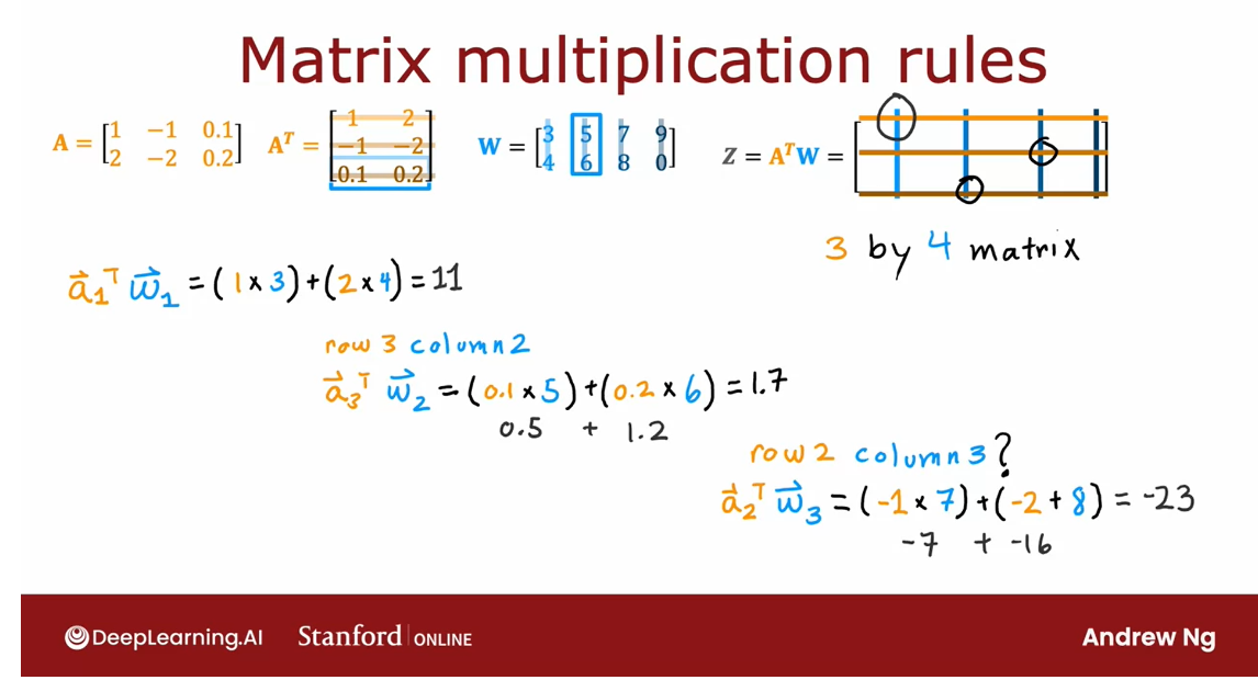
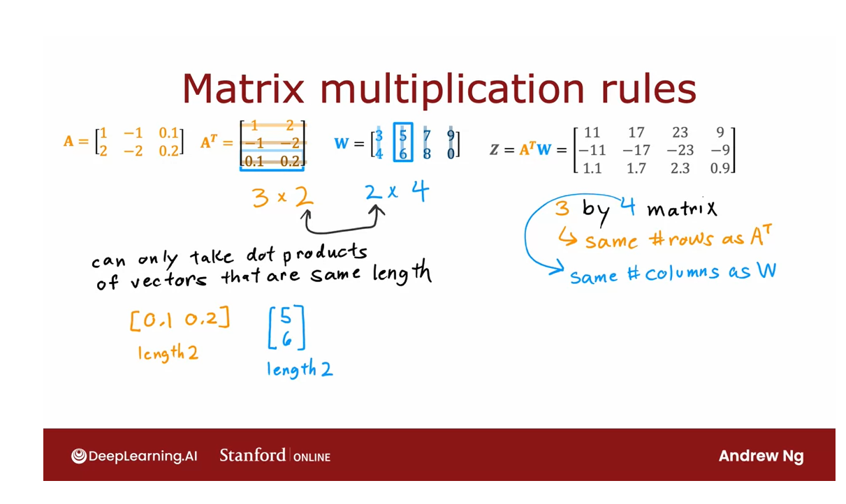
I just want to point out one
last interesting requirement for multiplying matrices together,
which is that X transpose here is a 3 by 2 matrix because
it has 3 rows and 2 columns, and W here is a 2 by 4 matrix because
it has 2 rows and 4 columns.

One requirement in order
to multiply two matrices together is that this number
must match that number.

And that’s because you can only take
dot products between vectors that are the same length.

So you can take the dot product
between a vector with two numbers. And that’s because you can take the inner
product between the vector of length 2 only with another vector of length 2. You can’t take the inner product between
vector of length 2 with a vector of length 3, for example.

And that’s why matrix multiplication
is valid only if the number of columns of the first matrix, that is
A transpose here is equal to the number of rolls of the second matrix,
that is the number of rolls of W here.

So that when you take dot
products during this process, you’re taking dot products
of vectors of the same size.

And then the other observation is that
the output Z equals a transpose, W. The dimensions of Z is 3 by 4. And so the output of this
multiplication will have the same number of rows as X transpose and
the same number of columns as W.

And so that too is another
property of matrix multiplication. So that’s matrix multiplication.

All these videos are optional. So thank you for
sticking with me through these.

And if you’re interested later in this
week, there are also some purely optional quizzes to let you practice some more
of these calculations yourself as well.

Some of that, let’s take what we’ve
learned about matrix multiplication and applied back to the vectorized
implementation of a Neural Network.

I have to say the first time I understood
the vectorized implementation, I thought that’s actually really cool. I’ve been implementing Neural Networks for awhile myself without
the vectorized implementation.

Andrew Ng: It ran blazingly much faster than anything I’ve done before

And when I finally understood
the vectorized implementation and implemented it that way for
the first time, it ran blazingly much faster than
anything I’ve ever done before.

And I thought, wow,
I wish I had figured this out earlier. The vectorized implementation,
it is a little bit complicated, but it makes your
networks run much faster. So let’s take a look at
that in the next video

Quiz

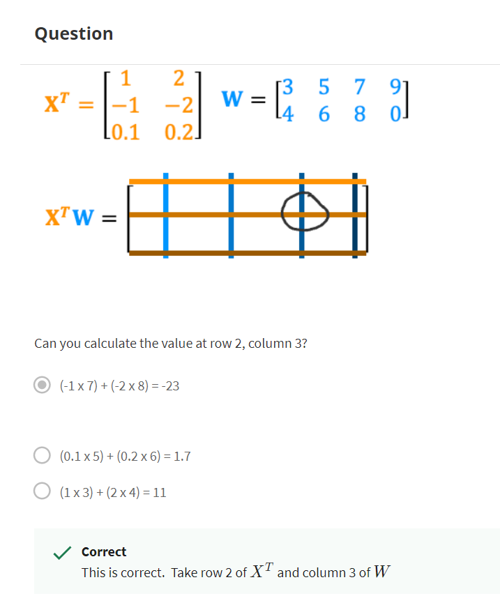
Matrix multiplication code

Without further ado,
let’s jump into the vectorize implementation
of a neural network. We’ll look at the code
that you have seen in a earlier video, and hopefully, Matmul, that is that matrix
multiplication calculation, will make more sense.
Let’s jump in.

You saw previously
how you can take the matrix A and compute A transpose times W resulting
in this matrix here, Z. In code if this is the matrix A, this is a NumPy array with the elements corresponding
to what I wrote on top, then A transpose, which
I’m going to write as AT, is going to be this matrix here, with again the columns of A
now laid out in rows instead.

By the way, instead of
setting up AT this way, another way to
compute AT in NumPy, we will write AT
equals A.T.

That’s the transpose
function that takes the columns of a matrix
and lays them on the side.

In code, here’s
how you initialize the matrix W as another
2D NumPy array. Then to compute Z equals
A transpose times W, you will write Z
equals np.matmul, AT, W, and that will compute
this matrix Z over here, giving you this
result down here.

By the way, if you
read other’s code, sometimes you see Z
equals AT and then the @ W. This is an alternative way of
calling the matmal function.

Although I find using
np.matmul to be clearer. The call you see in this class, we just use the
matmal function like this rather than this @.

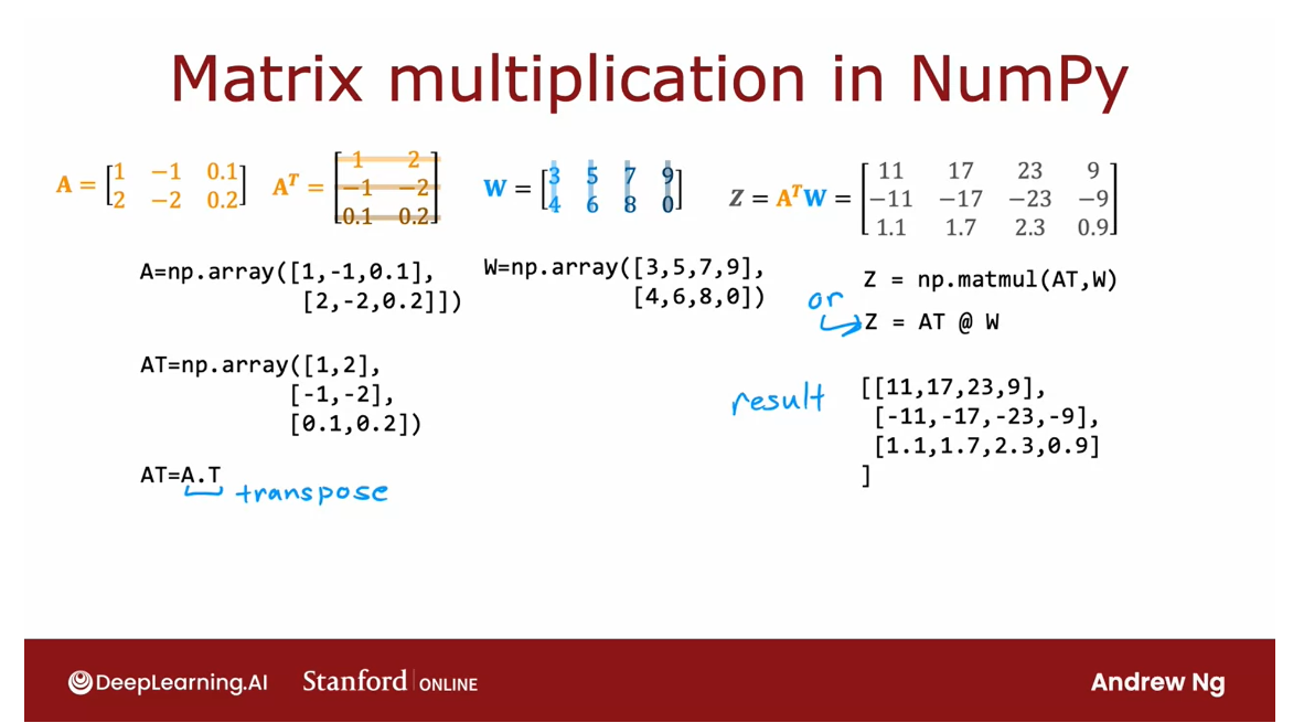
Vectorized implementation of forward prop

Let’s look at what a
vectorized implementation of forward prop looks like.

I’m going to set A
transpose to be equal to the input feature values 217. These are just the usual
input feature values, 200 degrees roasting
coffee for 17 minutes. This is a one by two matrix.

I’m going to take
the parameters w_1, w_2, and w_3, and stack them in columns
like this to form this matrix W. The values b_1, b_2, b_3, I’m going to put it into a one by three matrix, that is this matrix
B as follows.

Then it turns out that
if you were to compute Z equals A transpose W plus B, that will result in these three numbers and
that’s computed by taking the input feature values
and multiplying that by the first column and then
adding B to get 165.

Taking these feature values, dot-producting with
the second column, that is a weight w_2 and adding
b_2 to get negative 531. These feature values
dot product with the weights w_3 plus
b_3 to get 900.

Feel free to pause
the video if you wish to double-check
these calculations.

But this gives you is
the values of z^1_1, Z^1_2, and Z^1_3. Then finally, if the
function g applies the sigmoid function to these three numbers
element-wise, that is, applies the sigmoid
function to 165, to negative 531, and to 900, then you end up with A equals g of this matrix Z
ends up being 1,0,1. It’s 1,0,1 because sigmoid of 165 is so close to one that up to numerical round
off is based to one and these are bases 0 and 1.

Let’s look at how you
implement this in code.

Implement forward prop in code

A transpose is equal to this, is this one by two array of 217. The matrix W is this
two by three matrix, and B, this is one
by three matrix.

The way you can
implement forward prop in a layer is dense input A transpose W b is equal to z equals matmul A transpose
times W plus b. That just implements
this line of code.

Then a_out that is the output of this layer is equal to g, the activation function applied element-wise to this matrix Z.

You return a_out, and that gives you this value. In case you’re
comparing this slide with the slide a
few videos back, there was just one
little difference, which was by convention, the way this is
implemented in TensorFlow, rather than calling
this variable X,T, we call it just A, rather than calling
this variable A,T, we were calling it A_in, which is why this too is the correct implementation
of the code.

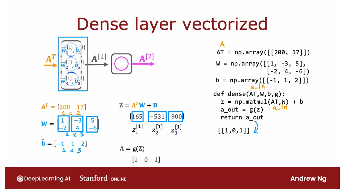
There is a convention
in TensorFlow that individual examples
are actually laid out in rows in the matrix X
rather than in the matrix X transpose which is why the code implementation actually looks like this in TensorFlow.

But this explains why with
just a few lines of code you can implement forward prop in the neural network and moreover, get a huge speed bonus because matmul matrix multiplication
can be done very efficiently using fast hardware and get a huge bonus because modern computers are very
good at implementing matrix multiplications such
as matmul efficiently.

That’s the last video this week. Thanks for sticking with
me all the way through the end of these
optional videos.

For the rest of this week, I hope you also take a look at the quizzes and the
practice labs and also the optional labs to exercise this material
even more deeply.

You now know how to do inference and forward prop in
a neural network, which I think is really
cool, so congratulations. After you have gone through
the quizzes and the labs, please also come back
and in the next week, we’ll look at how to actually
train a neural network. I look forward to
seeing you next week.

[11] Practice Lab: Neural networks

Programming Assignment: Neural Networks for Binary Classification

You have not submitted. You must earn 80/100 points to pass.

Instructions

Welcome to this first assignment of course 2. In this exercise, you will use a neural network to recognize the hand-written digits. You will first learn to build a neural network in a popular machine learning framework - Tensorflow. You will use your model to do image recognition on a portion of the famous MNIST data set. You will then learn what is ‘under the hood’ of these frameworks by implementing the forward path of the same network in NumPy in your own mini-framework.

Lab Content

Neural Networks for Handwritten Digit Recognition, Binary

In this exercise, you will use a neural network to recognize the hand-written digits zero and one.

Result: passed

Overview = Outline

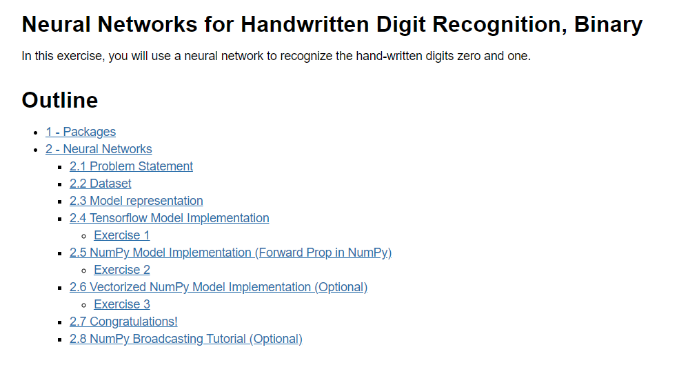
1 - Packages

First, let’s run the cell below to import all the packages that you will need during this assignment.

• numpy is the fundamental package for scientific computing with Python.
• matplotlib is a popular library to plot graphs in Python.
• tensorflow a popular platform for machine learning.

import numpy as np
import tensorflow as tf
from tensorflow.keras.models import Sequential
from tensorflow.keras.layers import Dense
import matplotlib.pyplot as plt
from autils import *
%matplotlib inline

import logging
logging.getLogger("tensorflow").setLevel(logging.ERROR)
tf.autograph.set_verbosity(0)

Tensorflow and Keras
Tensorflow is a machine learning package developed by Google. In 2019, Google integrated Keras into Tensorflow and released Tensorflow 2.0. Keras is a framework developed independently by François Chollet that creates a simple, layer-centric interface to Tensorflow. This course will be using the Keras interface.

2 - Neural Networks

In Course 1, you implemented logistic regression. This was extended to handle non-linear boundaries using polynomial regression. For even more complex scenarios such as image recognition, neural networks are preferred.

2.1 Problem Statement

In this exercise, you will use a neural network to recognize two handwritten digits, zero and one. This is a binary classification task. Automated handwritten digit recognition is widely used today - from recognizing zip codes (postal codes) on mail envelopes to recognizing amounts written on bank checks. You will extend this network to recognize all 10 digits (0-9) in a future assignment.

This exercise will show you how the methods you have learned can be used for this classification task.

2.2 Dataset

You will start by loading the dataset for this task.

• The load_data() function shown below loads the data into variables X and y

• The data set contains 1000 training examples of handwritten digits ${}^1$, here limited to zero and one.

  • Each training example is a 20-pixel x 20-pixel grayscale image of the digit.
    • Each pixel is represented by a floating-point number indicating the grayscale intensity at that location.
    • The 20 by 20 grid of pixels is “unrolled” into a 400-dimensional vector.
    • Each training example becomes a single row in our data matrix X.
    • This gives us a 1000 x 400 matrix X where every row is a training example of a handwritten digit image.

$$X=\left(\begin{array}{c}---(x^{(1)})---\\ ---(x^{(2)})---\\ ⋮\\ ---(x^{(m)})---\end{array}\right)$$

• The second part of the training set is a 1000 x 1 dimensional vector y that contains labels for the training set
  • y = 0 if the image is of the digit 0, y = 1 if the image is of the digit 1. _{This is a subset of the MNIST handwritten digit dataset (http://yann.lecun.com/exdb/mnist/)}

# load dataset
X, y = load_data()

2.2.1 View the variables

Let’s get more familiar with your dataset.

• A good place to start is to print out each variable and see what it contains.

The code below prints elements of the variables X and y.

print ('The first element of X is: ', X[0])

Output

The first element of X is:  [ 0.00000000e+00  0.00000000e+00  0.00000000e+00  0.00000000e+00
  0.00000000e+00  0.00000000e+00  0.00000000e+00  0.00000000e+00
  0.00000000e+00  0.00000000e+00  0.00000000e+00  0.00000000e+00
  0.00000000e+00  0.00000000e+00  0.00000000e+00  0.00000000e+00
  0.00000000e+00  0.00000000e+00  0.00000000e+00  0.00000000e+00
  0.00000000e+00  0.00000000e+00  0.00000000e+00  0.00000000e+00
  0.00000000e+00  0.00000000e+00  0.00000000e+00  0.00000000e+00
  0.00000000e+00  0.00000000e+00  0.00000000e+00  0.00000000e+00
  0.00000000e+00  0.00000000e+00  0.00000000e+00  0.00000000e+00
  0.00000000e+00  0.00000000e+00  0.00000000e+00  0.00000000e+00
  0.00000000e+00  0.00000000e+00  0.00000000e+00  0.00000000e+00
  0.00000000e+00  0.00000000e+00  0.00000000e+00  0.00000000e+00
  0.00000000e+00  0.00000000e+00  0.00000000e+00  0.00000000e+00
  0.00000000e+00  0.00000000e+00  0.00000000e+00  0.00000000e+00
  0.00000000e+00  0.00000000e+00  0.00000000e+00  0.00000000e+00
  0.00000000e+00  0.00000000e+00  0.00000000e+00  0.00000000e+00
  0.00000000e+00  0.00000000e+00  0.00000000e+00  8.56059680e-06
  1.94035948e-06 -7.37438725e-04 -8.13403799e-03 -1.86104473e-02
 -1.87412865e-02 -1.87572508e-02 -1.90963542e-02 -1.64039011e-02
 -3.78191381e-03  3.30347316e-04  1.27655229e-05  0.00000000e+00
  0.00000000e+00  0.00000000e+00  0.00000000e+00  0.00000000e+00
  0.00000000e+00  0.00000000e+00  1.16421569e-04  1.20052179e-04
 -1.40444581e-02 -2.84542484e-02  8.03826593e-02  2.66540339e-01
  2.73853746e-01  2.78729541e-01  2.74293607e-01  2.24676403e-01
  2.77562977e-02 -7.06315478e-03  2.34715414e-04  0.00000000e+00
  0.00000000e+00  0.00000000e+00  0.00000000e+00  0.00000000e+00
  0.00000000e+00  1.28335523e-17 -3.26286765e-04 -1.38651604e-02
  8.15651552e-02  3.82800381e-01  8.57849775e-01  1.00109761e+00
  9.69710638e-01  9.30928598e-01  1.00383757e+00  9.64157356e-01
  4.49256553e-01 -5.60408259e-03 -3.78319036e-03  0.00000000e+00
  0.00000000e+00  0.00000000e+00  0.00000000e+00  5.10620915e-06
  4.36410675e-04 -3.95509940e-03 -2.68537241e-02  1.00755014e-01
  6.42031710e-01  1.03136838e+00  8.50968614e-01  5.43122379e-01
  3.42599738e-01  2.68918777e-01  6.68374643e-01  1.01256958e+00
  9.03795598e-01  1.04481574e-01 -1.66424973e-02  0.00000000e+00
  0.00000000e+00  0.00000000e+00  0.00000000e+00  2.59875260e-05
 -3.10606987e-03  7.52456076e-03  1.77539831e-01  7.92890120e-01
  9.65626503e-01  4.63166079e-01  6.91720680e-02 -3.64100526e-03
 -4.12180405e-02 -5.01900656e-02  1.56102907e-01  9.01762651e-01
  1.04748346e+00  1.51055252e-01 -2.16044665e-02  0.00000000e+00
  0.00000000e+00  0.00000000e+00  5.87012352e-05 -6.40931373e-04
 -3.23305249e-02  2.78203465e-01  9.36720163e-01  1.04320956e+00
  5.98003217e-01 -3.59409041e-03 -2.16751770e-02 -4.81021923e-03
  6.16566793e-05 -1.23773318e-02  1.55477482e-01  9.14867477e-01
  9.20401348e-01  1.09173902e-01 -1.71058007e-02  0.00000000e+00
  0.00000000e+00  1.56250000e-04 -4.27724104e-04 -2.51466503e-02
  1.30532561e-01  7.81664862e-01  1.02836583e+00  7.57137601e-01
  2.84667194e-01  4.86865128e-03 -3.18688725e-03  0.00000000e+00
  8.36492601e-04 -3.70751123e-02  4.52644165e-01  1.03180133e+00
  5.39028101e-01 -2.43742611e-03 -4.80290033e-03  0.00000000e+00
  0.00000000e+00 -7.03635621e-04 -1.27262443e-02  1.61706648e-01
  7.79865383e-01  1.03676705e+00  8.04490400e-01  1.60586724e-01
 -1.38173339e-02  2.14879493e-03 -2.12622549e-04  2.04248366e-04
 -6.85907627e-03  4.31712963e-04  7.20680947e-01  8.48136063e-01
  1.51383408e-01 -2.28404366e-02  1.98971950e-04  0.00000000e+00
  0.00000000e+00 -9.40410539e-03  3.74520505e-02  6.94389110e-01
  1.02844844e+00  1.01648066e+00  8.80488426e-01  3.92123945e-01
 -1.74122413e-02 -1.20098039e-04  5.55215142e-05 -2.23907271e-03
 -2.76068376e-02  3.68645493e-01  9.36411169e-01  4.59006723e-01
 -4.24701797e-02  1.17356610e-03  1.88929739e-05  0.00000000e+00
  0.00000000e+00 -1.93511951e-02  1.29999794e-01  9.79821705e-01
  9.41862388e-01  7.75147704e-01  8.73632241e-01  2.12778350e-01
 -1.72353349e-02  0.00000000e+00  1.09937426e-03 -2.61793751e-02
  1.22872879e-01  8.30812662e-01  7.26501773e-01  5.24441863e-02
 -6.18971913e-03  0.00000000e+00  0.00000000e+00  0.00000000e+00
  0.00000000e+00 -9.36563862e-03  3.68349741e-02  6.99079299e-01
  1.00293583e+00  6.05704402e-01  3.27299224e-01 -3.22099249e-02
 -4.83053002e-02 -4.34069138e-02 -5.75151144e-02  9.55674190e-02
  7.26512627e-01  6.95366966e-01  1.47114481e-01 -1.20048679e-02
 -3.02798203e-04  0.00000000e+00  0.00000000e+00  0.00000000e+00
  0.00000000e+00 -6.76572712e-04 -6.51415556e-03  1.17339359e-01
  4.21948410e-01  9.93210937e-01  8.82013974e-01  7.45758734e-01
  7.23874268e-01  7.23341725e-01  7.20020340e-01  8.45324959e-01
  8.31859739e-01  6.88831870e-02 -2.77765012e-02  3.59136710e-04
  7.14869281e-05  0.00000000e+00  0.00000000e+00  0.00000000e+00
  0.00000000e+00  1.53186275e-04  3.17353553e-04 -2.29167177e-02
 -4.14402914e-03  3.87038450e-01  5.04583435e-01  7.74885876e-01
  9.90037446e-01  1.00769478e+00  1.00851440e+00  7.37905042e-01
  2.15455291e-01 -2.69624864e-02  1.32506127e-03  0.00000000e+00
  0.00000000e+00  0.00000000e+00  0.00000000e+00  0.00000000e+00
  0.00000000e+00  0.00000000e+00  0.00000000e+00  2.36366422e-04
 -2.26031454e-03 -2.51994485e-02 -3.73889910e-02  6.62121228e-02
  2.91134498e-01  3.23055726e-01  3.06260315e-01  8.76070942e-02
 -2.50581917e-02  2.37438725e-04  0.00000000e+00  0.00000000e+00
  0.00000000e+00  0.00000000e+00  0.00000000e+00  0.00000000e+00
  0.00000000e+00  0.00000000e+00  0.00000000e+00  0.00000000e+00
  0.00000000e+00  6.20939216e-18  6.72618320e-04 -1.13151411e-02
 -3.54641066e-02 -3.88214912e-02 -3.71077412e-02 -1.33524928e-02
  9.90964718e-04  4.89176960e-05  0.00000000e+00  0.00000000e+00
  0.00000000e+00  0.00000000e+00  0.00000000e+00  0.00000000e+00
  0.00000000e+00  0.00000000e+00  0.00000000e+00  0.00000000e+00
  0.00000000e+00  0.00000000e+00  0.00000000e+00  0.00000000e+00
  0.00000000e+00  0.00000000e+00  0.00000000e+00  0.00000000e+00
  0.00000000e+00  0.00000000e+00  0.00000000e+00  0.00000000e+00
  0.00000000e+00  0.00000000e+00  0.00000000e+00  0.00000000e+00
  0.00000000e+00  0.00000000e+00  0.00000000e+00  0.00000000e+00
  0.00000000e+00  0.00000000e+00  0.00000000e+00  0.00000000e+00
  0.00000000e+00  0.00000000e+00  0.00000000e+00  0.00000000e+00
  0.00000000e+00  0.00000000e+00  0.00000000e+00  0.00000000e+00
  0.00000000e+00  0.00000000e+00  0.00000000e+00  0.00000000e+00]

print ('The first element of y is: ', y[0,0])
print ('The last element of y is: ', y[-1,0])

Output

The first element of y is:  0
The last element of y is:  1

2.2.2 Check the dimensions of your variables

Another way to get familiar with your data is to view its dimensions. Please print the shape of X and y and see how many training examples you have in your dataset.

print ('The shape of X is: ' + str(X.shape))
print ('The shape of y is: ' + str(y.shape))

Output

The shape of X is: (1000, 400)
The shape of y is: (1000, 1)

2.2.3 Visualizing the Data

You will begin by visualizing a subset of the training set.

• In the cell below, the code randomly selects 64 rows from X, maps each row back to a 20 pixel by 20 pixel grayscale image and displays the images together.
• The label for each image is displayed above the image

import warnings
warnings.simplefilter(action='ignore', category=FutureWarning)
# You do not need to modify anything in this cell

m, n = X.shape

fig, axes = plt.subplots(8,8, figsize=(8,8))
fig.tight_layout(pad=0.1)

for i,ax in enumerate(axes.flat):
    # Select random indices
    random_index = np.random.randint(m)
    
    # Select rows corresponding to the random indices and
    # reshape the image
    X_random_reshaped = X[random_index].reshape((20,20)).T
    
    # Display the image
    ax.imshow(X_random_reshaped, cmap='gray')
    
    # Display the label above the image
    ax.set_title(y[random_index,0])
    ax.set_axis_off()

A part of the output

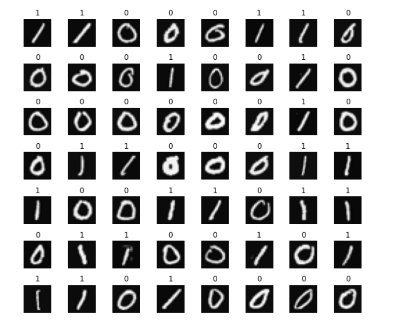
2.3 Model representation

The neural network you will use in this assignment is shown in the figure below.

• This has three dense layers with sigmoid activations.
  • Recall that our inputs are pixel values of digit images.
  • Since the images are of size $20\times 20$, this gives us $400$ inputs

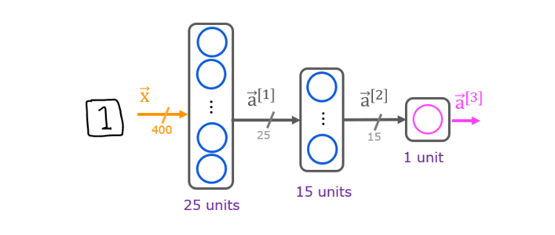
• The parameters have dimensions that are sized for a neural network with $25$ units in layer 1, $15$ units in layer 2 and $1$ output unit in layer 3.

  • Recall that the dimensions of these parameters are determined as follows:

    • If network has $s_{in}$ units in a layer and $s_{out}$ units in the next layer, then
      • $W$ will be of dimension $s_{in}\times s_{out}$.
      • $b$ will a vector with $s_{out}$ elements

  • Therefore, the shapes of W, and b, are

    • layer1: The shape of W1 is (400, 25) and the shape of b1 is (25,)
    • layer2: The shape of W2 is (25, 15) and the shape of b2 is: (15,)
    • layer3: The shape of W3 is (15, 1) and the shape of b3 is: (1,)

Note: The bias vector b could be represented as a 1-D (n,) or 2-D (n,1) array. Tensorflow utilizes a 1-D representation and this lab will maintain that convention.

Bias b 在 TensorFlow 中使用 1D 表示。

2.4 Tensorflow Model Implementation

Tensorflow models are built layer by layer. A layer’s input dimensions ($s_{in}$ above) are calculated for you. You specify a layer’s output dimensions and this determines the next layer’s input dimension. The input dimension of the first layer is derived from the size of the input data specified in the model.fit statment below.

Note: It is also possible to add an input layer that specifies the input dimension of the first layer. For example:
tf.keras.Input(shape=(400,)), #specify input shape
We will include that here to illuminate some model sizing.

Exercise 1

Below, using Keras Sequential model and Dense Layer with a sigmoid activation to construct the network described above.

# UNQ_C1
# GRADED CELL: Sequential model

model = Sequential(
    [               
        tf.keras.Input(shape=(400,)),    #specify input size
        ### START CODE HERE ### 
        Dense(25, activation="sigmoid"),
        Dense(15, activation="sigmoid"),
        Dense(1, activation="sigmoid")
        
        ### END CODE HERE ### 
    ], name = "my_model" 
)                            

使用

model.summary()

Output

Model: "my_model"
_________________________________________________________________
 Layer (type)                Output Shape              Param #   
=================================================================
 dense (Dense)               (None, 25)                10025     
                                                                 
 dense_1 (Dense)             (None, 15)                390       
                                                                 
 dense_2 (Dense)             (None, 1)                 16        
                                                                 
=================================================================
Total params: 10,431
Trainable params: 10,431
Non-trainable params: 0
_________________________________________________________________

Click to Expand

The model.summary() function displays a useful summary of the model. Because we have specified an input layer size, the shape of the weight and bias arrays are determined and the total number of parameters per layer can be shown. Note, the names of the layers may vary as they are auto-generated.

​

Model: "my_model"
_________________________________________________________________
Layer (type)                 Output Shape              Param #   
=================================================================
dense (Dense)                (None, 25)                10025     
_________________________________________________________________
dense_1 (Dense)              (None, 15)                390       
_________________________________________________________________
dense_2 (Dense)              (None, 1)                 16        
=================================================================
Total params: 10,431
Trainable params: 10,431
Non-trainable params: 0
_________________________________________________________________

Click for hints

As described in the lecture:

model = Sequential(                      
    [                                   
        tf.keras.Input(shape=(400,)),    # specify input size (optional)
        Dense(25, activation='sigmoid'), 
        Dense(15, activation='sigmoid'), 
        Dense(1,  activation='sigmoid')  
    ], name = "my_model"                                    
)                                       

下面是单元测试

# UNIT TESTS
from public_tests import * 

test_c1(model)

Output

All tests passed!

The parameter counts shown in the summary correspond to the number of elements in the weight and bias arrays as shown below.

L1_num_params = 400 * 25 + 25  # W1 parameters  + b1 parameters
L2_num_params = 25 * 15 + 15   # W2 parameters  + b2 parameters
L3_num_params = 15 * 1 + 1     # W3 parameters  + b3 parameters
print("L1 params = ", L1_num_params, ", L2 params = ", L2_num_params, ",  L3 params = ", L3_num_params )

Output

L1 params =  10025 , L2 params =  390 ,  L3 params =  16

Let’s further examine the weights to verify that tensorflow produced the same dimensions as we calculated above.

[layer1, layer2, layer3] = model.layers

#### Examine Weights shapes
W1,b1 = layer1.get_weights()
W2,b2 = layer2.get_weights()
W3,b3 = layer3.get_weights()
print(f"W1 shape = {W1.shape}, b1 shape = {b1.shape}")
print(f"W2 shape = {W2.shape}, b2 shape = {b2.shape}")
print(f"W3 shape = {W3.shape}, b3 shape = {b3.shape}")

Output

W1 shape = (400, 25), b1 shape = (25,)
W2 shape = (25, 15), b2 shape = (15,)
W3 shape = (15, 1), b3 shape = (1,)

Expected Output

W1 shape = (400, 25), b1 shape = (25,)  
W2 shape = (25, 15), b2 shape = (15,)  
W3 shape = (15, 1), b3 shape = (1,)

xx.get_weights returns a NumPy array. One can also access the weights directly in their tensor form. Note the shape of the tensors in the final layer.

print(model.layers[2].weights)

Output

[<tf.Variable 'dense_2/kernel:0' shape=(15, 1) dtype=float32, numpy=
array([[-0.17152691],
       [ 0.0448547 ],
       [ 0.5435689 ],
       [-0.19693327],
       [-0.10491323],
       [-0.12440932],
       [-0.16279677],
       [ 0.5802497 ],
       [-0.43265766],
       [-0.19242433],
       [ 0.08558798],
       [ 0.4026435 ],
       [-0.5408892 ],
       [ 0.2926998 ],
       [-0.00211334]], dtype=float32)>, <tf.Variable 'dense_2/bias:0' shape=(1,) dtype=float32, numpy=array([0.], dtype=float32)>]

The following code will define a loss function and run gradient descent to fit the weights of the model to the training data. This will be explained in more detail in the following week.

model.compile(
    loss=tf.keras.losses.BinaryCrossentropy(),
    optimizer=tf.keras.optimizers.Adam(0.001),
)

model.fit(
    X,y,
    epochs=20
)

Output

Epoch 1/20
32/32 [==============================] - 0s 1ms/step - loss: 0.6136
Epoch 2/20
32/32 [==============================] - 0s 1ms/step - loss: 0.4725
Epoch 3/20
32/32 [==============================] - 0s 2ms/step - loss: 0.3350
Epoch 4/20
32/32 [==============================] - 0s 1ms/step - loss: 0.2345
Epoch 5/20
32/32 [==============================] - 0s 2ms/step - loss: 0.1704
Epoch 6/20
32/32 [==============================] - 0s 1ms/step - loss: 0.1297
Epoch 7/20
32/32 [==============================] - 0s 2ms/step - loss: 0.1029
Epoch 8/20
32/32 [==============================] - 0s 2ms/step - loss: 0.0840
Epoch 9/20
32/32 [==============================] - 0s 1ms/step - loss: 0.0702
Epoch 10/20
32/32 [==============================] - 0s 2ms/step - loss: 0.0601
Epoch 11/20
32/32 [==============================] - 0s 1ms/step - loss: 0.0523
Epoch 12/20
32/32 [==============================] - 0s 2ms/step - loss: 0.0462
Epoch 13/20
32/32 [==============================] - 0s 1ms/step - loss: 0.0413
Epoch 14/20
32/32 [==============================] - 0s 2ms/step - loss: 0.0374
Epoch 15/20
32/32 [==============================] - 0s 2ms/step - loss: 0.0340
Epoch 16/20
32/32 [==============================] - 0s 1ms/step - loss: 0.0313
Epoch 17/20
32/32 [==============================] - 0s 2ms/step - loss: 0.0289
Epoch 18/20
32/32 [==============================] - 0s 1ms/step - loss: 0.0268
Epoch 19/20
32/32 [==============================] - 0s 2ms/step - loss: 0.0251
Epoch 20/20
32/32 [==============================] - 0s 1ms/step - loss: 0.0235

Out[20]:

<keras.callbacks.History at 0x7f5619686110>

To run the model on an example to make a prediction, use Keras predict. The input to predict is an array so the single example is reshaped to be two dimensional.

prediction = model.predict(X[0].reshape(1,400))  # a zero
print(f" predicting a zero: {prediction}")
prediction = model.predict(X[500].reshape(1,400))  # a one
print(f" predicting a one:  {prediction}")

Output

predicting a zero: [[0.01485184]]
predicting a one:  [[0.97910416]]

如果对于predict函数的输入，不进行 reshape 会怎样呢？

以下是测试代码，即错误代码

prediction = model.predict(X[0])  # a zero
print(f" predicting a zero: {prediction}")
prediction = model.predict(X[500].reshape(1,400))  # a one
print(f" predicting a one:  {prediction}")

报错如下，维数不兼容，需要的是2D，输入的却是1D，所以会报错。因此我们需要reshape一下。

ValueError: Exception encountered when calling layer "my_model" (type Sequential).

Input 0 of layer "dense" is incompatible with the layer: expected min_ndim=2, found ndim=1. Full shape received: (None,)

Call arguments received:
  • inputs=tf.Tensor(shape=(None,), dtype=float32)
  • training=False
  • mask=None

The output of the model is interpreted as a probability. In the first example above, the input is a zero. The model predicts the probability that the input is a one is nearly zero.
In the second example, the input is a one. The model predicts the probability that the input is a one is nearly one.
As in the case of logistic regression, the probability is compared to a threshold to make a final prediction.

if prediction >= 0.5:
    yhat = 1
else:
    yhat = 0
print(f"prediction after threshold: {yhat}")

Output

prediction after threshold: 1

Let’s compare the predictions vs the labels for a random sample of 64 digits. This takes a moment to run.

import warnings
warnings.simplefilter(action='ignore', category=FutureWarning)
# You do not need to modify anything in this cell

m, n = X.shape

fig, axes = plt.subplots(8,8, figsize=(8,8))
fig.tight_layout(pad=0.1,rect=[0, 0.03, 1, 0.92]) #[left, bottom, right, top]

for i,ax in enumerate(axes.flat):
    # Select random indices
    random_index = np.random.randint(m)
    
    # Select rows corresponding to the random indices and
    # reshape the image
    X_random_reshaped = X[random_index].reshape((20,20)).T
    
    # Display the image
    ax.imshow(X_random_reshaped, cmap='gray')
    
    # Predict using the Neural Network
    prediction = model.predict(X[random_index].reshape(1,400))
    if prediction >= 0.5:
        yhat = 1
    else:
        yhat = 0
    
    # Display the label above the image
    ax.set_title(f"{y[random_index,0]},{yhat}")
    ax.set_axis_off()
fig.suptitle("Label, yhat", fontsize=16)
plt.show()

Output

2.5 NumPy Model Implementation (Forward Prop in NumPy)

As described in lecture, it is possible to build your own dense layer using NumPy. This can then be utilized to build a multi-layer neural network.

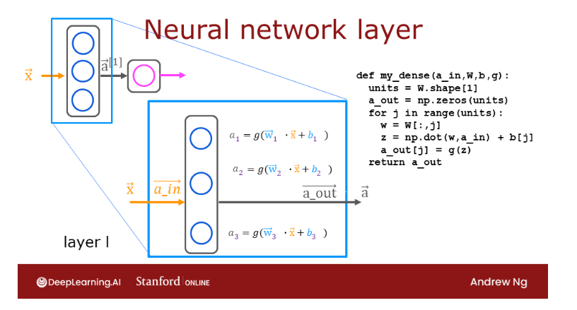
Exercise 2

Below, build a dense layer subroutine. The example in lecture utilized a for loop to visit each unit (j) in the layer and perform the dot product of the weights for that unit (W[:,j]) and sum the bias for the unit (b[j]) to form z. An activation function g(z) is then applied to that result. This section will not utilize some of the matrix operations described in the optional lectures. These will be explored in a later section.

# UNQ_C2
# GRADED FUNCTION: my_dense

def my_dense(a_in, W, b, g):
    """
    Computes dense layer
    Args:
      a_in (ndarray (n, )) : Data, 1 example 
      W    (ndarray (n,j)) : Weight matrix, n features per unit, j units
      b    (ndarray (j, )) : bias vector, j units  
      g    activation function (e.g. sigmoid, relu..)
    Returns
      a_out (ndarray (j,))  : j units
    """
    units = W.shape[1]
    a_out = np.zeros(units)
### START CODE HERE ### 
    for j in range(units):
        w = W[:,j]
        z = np.dot(w, a_in) + b[j]
        a_out[j] = g(z)
        
### END CODE HERE ### 
    return(a_out)

自测

# Quick Check
x_tst = 0.1*np.arange(1,3,1).reshape(2,)  # (1 examples, 2 features)
W_tst = 0.1*np.arange(1,7,1).reshape(2,3) # (2 input features, 3 output features)
b_tst = 0.1*np.arange(1,4,1).reshape(3,)  # (3 features)
A_tst = my_dense(x_tst, W_tst, b_tst, sigmoid)
print(A_tst)

Output

[0.54735762 0.57932425 0.61063923]

Expected Output

[0.54735762 0.57932425 0.61063923]

Numpy 中 arrange的用法： https://blog.csdn.net/qq_41800366/article/details/86589680

numpy.arange(start, stop, step, dtype = None)

在给定间隔内返回均匀间隔的值。

值在半开区间 [开始，停止]内生成（换句话说，包括开始但不包括停止的区间）,返回的是 ndarray 。

Click for hints

As described in the lecture:

def my_dense(a_in, W, b, g):
    """
    Computes dense layer
    Args:
      a_in (ndarray (n, )) : Data, 1 example 
      W    (ndarray (n,j)) : Weight matrix, n features per unit, j units
      b    (ndarray (j, )) : bias vector, j units  
      g    activation function (e.g. sigmoid, relu..)
    Returns
      a_out (ndarray (j,))  : j units
    """
    units = W.shape[1]
    a_out = np.zeros(units)
    for j in range(units):             
        w =                            # Select weights for unit j. These are in column j of W
        z =                            # dot product of w and a_in + b
        a_out[j] =                     # apply activation to z
    return(a_out)

​ Click for more hints

def my_dense(a_in, W, b, g):
    """
    Computes dense layer
    Args:
      a_in (ndarray (n, )) : Data, 1 example 
      W    (ndarray (n,j)) : Weight matrix, n features per unit, j units
      b    (ndarray (j, )) : bias vector, j units  
      g    activation function (e.g. sigmoid, relu..)
    Returns
      a_out (ndarray (j,))  : j units
    """
    units = W.shape[1]
    a_out = np.zeros(units)
    for j in range(units):             
        w = W[:,j]                     
        z = np.dot(w, a_in) + b[j]     
        a_out[j] = g(z)                
    return(a_out)

单元测试

# UNIT TESTS
test_c2(my_dense)

Output

All tests passed!

The following cell builds a three-layer neural network utilizing the my_dense subroutine above.

def my_sequential(x, W1, b1, W2, b2, W3, b3):
    a1 = my_dense(x,  W1, b1, sigmoid)
    a2 = my_dense(a1, W2, b2, sigmoid)
    a3 = my_dense(a2, W3, b3, sigmoid)
    return(a3)

We can copy trained weights and biases from Tensorflow.

W1_tmp,b1_tmp = layer1.get_weights()
W2_tmp,b2_tmp = layer2.get_weights()
W3_tmp,b3_tmp = layer3.get_weights()

Make predictions

# make predictions
prediction = my_sequential(X[0], W1_tmp, b1_tmp, W2_tmp, b2_tmp, W3_tmp, b3_tmp )
if prediction >= 0.5:
    yhat = 1
else:
    yhat = 0
print( "yhat = ", yhat, " label= ", y[0,0])
prediction = my_sequential(X[500], W1_tmp, b1_tmp, W2_tmp, b2_tmp, W3_tmp, b3_tmp )
if prediction >= 0.5:
    yhat = 1
else:
    yhat = 0
print( "yhat = ", yhat, " label= ", y[500,0])

Output

yhat =  0  label=  0
yhat =  1  label=  1

Run the following cell to see predictions from both the Numpy model and the Tensorflow model. This takes a moment to run.

import warnings
warnings.simplefilter(action='ignore', category=FutureWarning)
# You do not need to modify anything in this cell

m, n = X.shape

fig, axes = plt.subplots(8,8, figsize=(8,8))
fig.tight_layout(pad=0.1,rect=[0, 0.03, 1, 0.92]) #[left, bottom, right, top]

for i,ax in enumerate(axes.flat):
    # Select random indices
    random_index = np.random.randint(m)
    
    # Select rows corresponding to the random indices and
    # reshape the image
    X_random_reshaped = X[random_index].reshape((20,20)).T
    
    # Display the image
    ax.imshow(X_random_reshaped, cmap='gray')

    # Predict using the Neural Network implemented in Numpy
    my_prediction = my_sequential(X[random_index], W1_tmp, b1_tmp, W2_tmp, b2_tmp, W3_tmp, b3_tmp )
    my_yhat = int(my_prediction >= 0.5)

    # Predict using the Neural Network implemented in Tensorflow
    tf_prediction = model.predict(X[random_index].reshape(1,400))
    tf_yhat = int(tf_prediction >= 0.5)
    
    # Display the label above the image
    ax.set_title(f"{y[random_index,0]},{tf_yhat},{my_yhat}")
    ax.set_axis_off() 
fig.suptitle("Label, yhat Tensorflow, yhat Numpy", fontsize=16)
plt.show()

Output

2.6 Vectorized NumPy Model Implementation (Optional)

The optional lectures described vector and matrix operations that can be used to speed the calculations.
Below describes a layer operation that computes the output for all units in a layer on a given input example:

We can demonstrate this using the examples X and the W1,b1 parameters above. We use np.matmul to perform the matrix multiply. Note, the dimensions of x and W must be compatible as shown in the diagram above.

x = X[0].reshape(-1,1)         # column vector (400,1)
z1 = np.matmul(x.T,W1) + b1    # (1,400)(400,25) = (1,25)
a1 = sigmoid(z1)
print(a1.shape)

Output

(1, 25)

reshape(-1, 1) 是什么意思？ -1是自动推导，比如原来的shape 是 3 x 4，现在经过 reshape(-1, 1)，这里显示指出是1列，那是多少行呢？这是reshape自动计算的。 于是这里变成 12 x 1的shape。

所以 reshape 中的 -1 是由shape进行的自动推导，一般由全部维数和其他维数已知，方可进行自动推导。

You can take this a step further and compute all the units for all examples in one Matrix-Matrix operation.

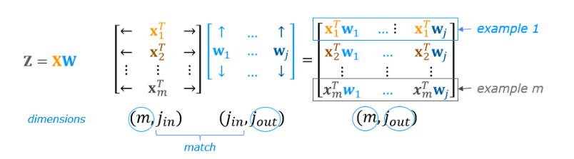
The full operation is $\mathbf{Z}=\mathbf{XW}+\mathbf{b}$. This will utilize NumPy broadcasting to expand $\mathbf{b}$ to $m$ rows. If this is unfamiliar, a short tutorial is provided at the end of the notebook.

Exercise 3

Reference

Below, compose a new my_dense_v subroutine that performs the layer calculations for a matrix of examples. This will utilize np.matmul().

# UNQ_C3
# GRADED FUNCTION: my_dense_v

def my_dense_v(A_in, W, b, g):
    """
    Computes dense layer
    Args:
      A_in (ndarray (m,n)) : Data, m examples, n features each
      W    (ndarray (n,j)) : Weight matrix, n features per unit, j units
      b    (ndarray (j,1)) : bias vector, j units  
      g    activation function (e.g. sigmoid, relu..)
    Returns
      A_out (ndarray (m,j)) : m examples, j units
    """
### START CODE HERE ### 
    Z = np.matmul(A_in, W) + b
    A_out = g(Z)
    
### END CODE HERE ### 
    return(A_out)

Test

X_tst = 0.1*np.arange(1,9,1).reshape(4,2) # (4 examples, 2 features)
W_tst = 0.1*np.arange(1,7,1).reshape(2,3) # (2 input features, 3 output features)
b_tst = 0.1*np.arange(1,4,1).reshape(1,3) # (3 features, 1)
A_tst = my_dense_v(X_tst, W_tst, b_tst, sigmoid)
print(A_tst)

Output

tf.Tensor(
[[0.54735762 0.57932425 0.61063923]
 [0.57199613 0.61301418 0.65248946]
 [0.5962827  0.64565631 0.6921095 ]
 [0.62010643 0.67699586 0.72908792]], shape=(4, 3), dtype=float64)

Expected Output

[[0.54735762 0.57932425 0.61063923]
 [0.57199613 0.61301418 0.65248946]
 [0.5962827  0.64565631 0.6921095 ]
 [0.62010643 0.67699586 0.72908792]]

Click for hints

In matrix form, this can be written in one or two lines.

   Z = np.matmul of A_in and W plus b    
   A_out is g(Z)  

Click for code

def my_dense_v(A_in, W, b, g):
    """
    Computes dense layer
    Args:
      A_in (ndarray (m,n)) : Data, m examples, n features each
      W    (ndarray (n,j)) : Weight matrix, n features per unit, j units
      b    (ndarray (j,1)) : bias vector, j units  
      g    activation function (e.g. sigmoid, relu..)
    Returns
      A_out (ndarray (m,j)) : m examples, j units
    """
    Z = np.matmul(A_in,W) + b    
    A_out = g(Z)                 
    return(A_out)

Unit test

# UNIT TESTS
test_c3(my_dense_v)

Output

All tests passed!

The following cell builds a three-layer neural network utilizing the my_dense_v subroutine above.

def my_sequential_v(X, W1, b1, W2, b2, W3, b3):
    A1 = my_dense_v(X,  W1, b1, sigmoid)
    A2 = my_dense_v(A1, W2, b2, sigmoid)
    A3 = my_dense_v(A2, W3, b3, sigmoid)
    return(A3)

We can again copy trained weights and biases from Tensorflow.

W1_tmp,b1_tmp = layer1.get_weights()
W2_tmp,b2_tmp = layer2.get_weights()
W3_tmp,b3_tmp = layer3.get_weights()

Let’s make a prediction with the new model. This will make a prediction on all of the examples at once. Note the shape of the output.

Prediction = my_sequential_v(X, W1_tmp, b1_tmp, W2_tmp, b2_tmp, W3_tmp, b3_tmp )
Prediction.shape

Output

TensorShape([1000, 1])

We’ll apply a threshold of 0.5 as before, but to all predictions at once.

Yhat = (Prediction >= 0.5).numpy().astype(int)
print("predict a zero: ",Yhat[0], "predict a one: ", Yhat[500])

Output

predict a zero:  [0] predict a one:  [1]

Run the following cell to see predictions. This will use the predictions we just calculated above. This takes a moment to run.

import warnings
warnings.simplefilter(action='ignore', category=FutureWarning)
# You do not need to modify anything in this cell

m, n = X.shape

fig, axes = plt.subplots(8, 8, figsize=(8, 8))
fig.tight_layout(pad=0.1, rect=[0, 0.03, 1, 0.92]) #[left, bottom, right, top]

for i, ax in enumerate(axes.flat):
    # Select random indices
    random_index = np.random.randint(m)
    
    # Select rows corresponding to the random indices and
    # reshape the image
    X_random_reshaped = X[random_index].reshape((20, 20)).T
    
    # Display the image
    ax.imshow(X_random_reshaped, cmap='gray')
   
    # Display the label above the image
    ax.set_title(f"{y[random_index,0]}, {Yhat[random_index, 0]}")
    ax.set_axis_off() 
fig.suptitle("Label, Yhat", fontsize=16)
plt.show()

Output

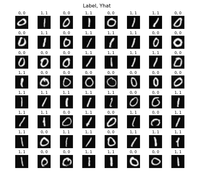
You can see how one of the misclassified images looks.

fig = plt.figure(figsize=(1, 1))
errors = np.where(y != Yhat)
random_index = errors[0][0]
X_random_reshaped = X[random_index].reshape((20, 20)).T
plt.imshow(X_random_reshaped, cmap='gray')
plt.title(f"{y[random_index,0]}, {Yhat[random_index, 0]}")
plt.axis('off')
plt.show()

Output

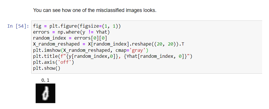
2.7 Congratulations!

You have successfully built and utilized a neural network.

2.8 NumPy Broadcasting Tutorial (Optional)

In the last example, $\mathbf{Z}=\mathbf{XW}+\mathbf{b}$ utilized NumPy broadcasting to expand the vector $\mathbf{b}$. If you are not familiar with NumPy Broadcasting, this short tutorial is provided.

$\mathbf{XW}$ is a matrix-matrix operation with dimensions $(m,j_1)(j_1,j_2)$ which results in a matrix with dimension $(m,j_2)$. To that, we add a vector $\mathbf{b}$ with dimension $(j_2,)$. $\mathbf{b}$ must be expanded to be a $(m,j_2)$ matrix for this element-wise operation to make sense. This expansion is accomplished for you by NumPy broadcasting.

Broadcasting applies to element-wise operations.
Its basic operation is to ‘stretch’ a smaller dimension by replicating elements to match a larger dimension.

More specifically:
When operating on two arrays, NumPy compares their shapes element-wise. It starts with the trailing (i.e. rightmost) dimensions and works its way left. Two dimensions are compatible when

• they are equal, or
• one of them is 1

If these conditions are not met, a ValueError: operands could not be broadcast together exception is thrown, indicating that the arrays have incompatible shapes. The size of the resulting array is the size that is not 1 along each axis of the inputs.

Here are some examples:

The graphic below describes expanding dimensions. Note the red text below:

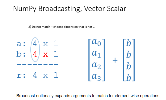
The graphic above shows NumPy expanding the arguments to match before the final operation. Note that this is a notional description. The actual mechanics of NumPy operation choose the most efficient implementation.

For each of the following examples, try to guess the size of the result before running the example.

a = np.array([1,2,3]).reshape(-1,1)  #(3,1)
b = 5
print(f"(a + b).shape: {(a + b).shape}, \na + b = \n{a + b}")

Output

(a + b).shape: (3, 1), 
a + b = 
[[6]
 [7]
 [8]]

Note that this applies to all element-wise operations:

a = np.array([1,2,3]).reshape(-1,1)  #(3,1)
b = 5
print(f"(a * b).shape: {(a * b).shape}, \na * b = \n{a * b}")

Output

(a * b).shape: (3, 1), 
a * b = 
[[ 5]
 [10]
 [15]]

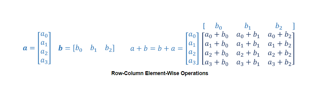
a = np.array([1,2,3,4]).reshape(-1,1) # (4, 1)
b = np.array([1,2,3]).reshape(1,-1)   # (1, 3)
print(a)
print(b)
# a + b => (4, 3)
print(f"(a + b).shape: {(a + b).shape}, \na + b = \n{a + b}")

Output

[[1]
 [2]
 [3]
 [4]]
[[1 2 3]]
(a + b).shape: (4, 3), 
a + b = 
[[2 3 4]
 [3 4 5]
 [4 5 6]
 [5 6 7]]

This is the scenario in the dense layer you built above. Adding a 1-D vector $b$ to a (m,j) matrix.

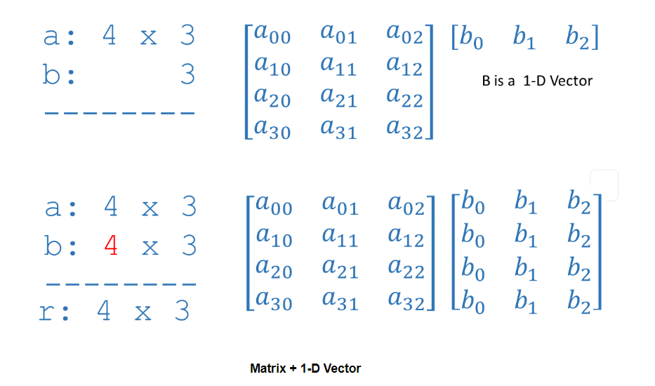
其他

commit

git commit -m "Finish xxx part of week xx of Advanced Learning Algorithms"

For example

git commit -m "Finish 'Forward prop in a single layer' and 'General implementation of forward propagation' part of week 01 of Advanced Learning Algorithms"

git commit -m "Finish 'Practice Lab: Neural Networks for Handwritten Digit Recognition, Binary' part of week 01 of Advanced Learning Algorithms"

Without formatting

git commit -m "Finish Practice quiz: Neural network model part of week 01 of Advanced Learning Algorithms, without formating the transcript"

Reformat transcript

 git commit -m "Reformat learning notes of Example: Recognizing Images part of week 01 of Advanced Learning Algorithms"

Course name:

Advanced Learning Algorithms

英文发音

rewind this video：重放此视频

not counting the input layer: 不计算（计数）输入层

subroutine: 子程序

向量转置：taking the first column of A and laying it on the side like this: 把这一列变成一行

string together: 串起来

underscore : 下划线

double square bracket: [[ ]]

coffee roasting: 咖啡烘焙

is getting a little bit cluttered: 变得杂乱无章

方括号：square bracket, []

superscript in square brackets 1: 上标是方括号1,[1]

carry out this task: 做这个任务

Biological neuron:

nucleus of the neuron: 神经元核

dendrites: 树突 ˈdendrīt

axon：轴突 ˈakˌsän

make inroads into 有巨大的影响力；取得进步

From Longman Dictionary of Contemporary English

make inroads into/on something

• to have an important effect or influence on something, especially by taking something away from it

Video is making huge inroads into attendance figures at movie theaters (=taking away its customers).

They have made significant inroads into the European market.

The administrative workload is making massive inroads into our working day (=taking away time).

• to make some progress towards achieving something difficult

We haven’t made much of an inroad into the backlog of work.

they gained in popularity again：火了

it fell out of favor for a while: 失宠了一段时间

10 to the power of 10: $10^{10}$

diagnose: ˌdīəɡˈnōs 诊断，确诊

convex: 凸的 ˌkänˈveks， 重音在后

e to the negative z: $e^{-z}$

hammock: 吊床 ˈhamək

square of xxx: xxx的平方

parabola: 抛物线， pəˈrabələ

---

1. 1 ↩︎

2. 1 ↩︎

3. 1 ↩︎

4. 2 ↩︎