【论文阅读】Bayes’ Rays:神经辐射场的不确定性量化
- 1. Introduction
- 2. Related work
- 3. Background
- 3.2. Neural Laplace Approximations
- 4. Method
- 4.1. Intuition
- 4.2. Modeling perturbations
- 4.3. Approximating H
- 4.4. Spatial uncertainty
- 5. Experiments & Applications
- 5.1. Uncertainty Evaluation – Figures 6
- 5.2. NeRF Clean Up – Figures 1 and 4
- 5.3. Algorithmic ablations – Figures 3, 5 and 8
- 6. Conclusions
 Bayes’ Rays: Uncertainty Quantification for Neural Radiance Fields
Neural Radiance Fields (NeRFs) have shown promise in applications like view synthesis and depth estimation, but learning from multiview images faces inherent uncertainties. Current methods to quantify them are either heuristic or computationally demanding. We introduce BayesRays, a post-hoc framework to evaluate uncertainty in any pretrained NeRF without modifying the training process. Our method establishes a volumetric uncertainty field using spatial perturbations and a Bayesian Laplace approximation. We derive our algorithm statistically and show its superior performance in key metrics and applications. Additional results available at: https://bayesrays.github.io
神经辐射场(NeRF)在视图合成和深度估计等应用中显示出了前景,但从多视图图像中学习面临着固有的不确定性。目前量化它们的方法要么是启发式的1,要么是计算要求较高的。我们引入了 BayesRays,这是一个事后框架,可以在不修改训练过程的情况下评估任何预训练 NeRF 中的不确定性。我们的方法使用空间扰动和贝叶斯拉普拉斯近似建立体积不确定性场。我们以统计方式推导我们的算法,并在关键指标和应用中展示其卓越的性能。其他结果请访问:https://bayesrays.github.io

图 1.我们引入了 BayesRays,这是一种事后算法,用于估计任何任意架构的任何预训练 NeRF 的空间不确定性。我们的方法不需要额外的训练,并且可以用来清理由遮挡或不完整的数据引起的 NeRF 伪影。
1. Introduction
Neural Radiance Fields (NeRFs) have shown promise in applications like view synthesis and depth estimation, but learning from multiview images faces inherent uncertainties. Current methods to quantify them are either heuristic or computationally demanding. We introduce BayesRays, a post-hoc framework to evaluate uncertainty in any pretrained NeRF without modifying the training process. Our method establishes a volumetric uncertainty field using spatial perturbations and a Bayesian Laplace approximation. We derive our algorithm statistically and show its superior performance in key metrics and applications. Additional results available at: https://bayesrays.github.io
神经辐射场(NeRF)在视图合成和深度估计等应用中显示出了前景,但从多视图图像中学习面临着固有的不确定性。目前量化它们的方法要么是启发式的,要么是计算要求较高的。我们引入了 BayesRays,这是一个事后框架,可以在不修改训练过程的情况下评估任何预训练 NeRF 中的不确定性。我们的方法使用空间扰动和贝叶斯拉普拉斯近似建立体积不确定性场。我们以统计方式推导我们的算法,并在关键指标和应用中展示其卓越的性能。其他结果请访问:https://bayesrays.github.io
Neural Radiance Fields (NeRFs) are a class of learned volumetric implicit scene representations that have exploded in popularity due to their success in applications like novel view synthesis and depth estimation. The process of learning a NeRF from a discrete set of multiview images is plagued with uncertainty: even in perfect experimental conditions, occlusions and missing views will limit the epistemic knowledge that the model can acquire about the scene.
神经辐射场 (NeRF) 是一类学习的体积隐式场景表示,由于其在新颖的视图合成和深度估计等应用中的成功而受到广泛欢迎 。从一组离散的多视图图像中学习 NeRF 的过程充满了不确定性:即使在完美的实验条件下,遮挡和缺失的视图也会限制模型可以获得的有关场景的认知知识。
Studying the epistemic uncertainty in NeRF is fundamental for tasks like outlier detection [21] and next-best-view planning [31] that expand NeRF’s performance and application domain to critical areas like autonomous driving [11]. However, quantifying the uncertainty contained in a NeRF model is a relatively new area of study, with existing methods proposing either heuristic proxies without theoretical guarantees [14, 58] or probabilistic techniques that require costly computational power [47] and/or elaborate changes to the conventional NeRF training pipeline [41, 42].
研究 NeRF 中的认知不确定性对于异常值检测 [21] 和次最佳视图规划 [31] 等任务至关重要,这些任务将 NeRF 的性能和应用领域扩展到自动驾驶等关键领域 [11]。然而,量化 NeRF 模型中包含的不确定性是一个相对较新的研究领域,现有方法提出要么没有理论保证的启发式代理 [14, 58],要么需要昂贵的计算能力 [47] 和/或对传统的 NeRF 训练流程 进行精心改动[41, 42]。
We draw inspiration from triangulation problems in classic photogrammetry [45], where uncertainty is often modeled through distributions of feature point positions in image space that are then projected onto 3D (see Figure 2). Intuitively, this distribution measures how much a feature’s position can be perturbed while maintaining multi-view consistency. We apply a similar intuition to NeRF, identifying the regions of the radiance field that can be spatially perturbed with minimal impact on the reconstruction loss.
我们从经典摄影测量中的三角测量问题中汲取灵感 [45],其中不确定性通常通过图像空间中特征点位置的分布进行建模,然后投影到 3D 上(见图 2)。直观上,这种分布衡量了在保持多视图一致性的同时,特征的位置可以受到多大程度的扰动。我们将类似的直觉应用于 NeRF,识别可以在空间上扰动且对重建损失影响最小的辐射场区域。

图 2. 受到经典摄影测量中不确定性量化(左)的启发,我们在 NeRF 中发现了认知不确定性(右)。
We propose BayesRays, a post-hoc framework for quantifying the uncertainty of any arbitrary pre-trained NeRF. Without requiring any changes to the training pipeline and regardless of the architecture in use in the given NeRF (see Figure 3), our method simulates spatially parametrized perturbations of the radiance field and uses a Bayesian Laplace approximation to produce a volumetric uncertainty field, which can be rendered like an additional color channel.
我们提出了 BayesRays,一个用于量化任何任意预训练 NeRF 的不确定性的事后框架。无需对训练流程进行任何更改,并且无论给定 NeRF 中使用的架构如何(见图 3),我们的方法都会模拟辐射场的空间参数化扰动,并使用贝叶斯拉普拉斯近似来生成体积不确定性场,这可以像附加颜色通道一样渲染。

图 3.BayesRays 应用于不同的 NeRF 架构。 “lego”[24]仅使用其左半球上的相片进行机训练。
In this work, we show that our calculated uncertainties are not only statistically meaningful but also outperform previous works on key metrics like correlation to reconstructed depth error. Furthermore, they provide a framework for critical applications like removing floater artifacts from NeRF, matching or improving the state-of-the-art (see Figure 1). In summary, our main contributions are:
在这项工作中,我们表明,我们计算的不确定性不仅具有统计意义,而且在关键指标(例如与重建深度误差的相关性)方面优于以前的工作。此外,它们还为关键应用程序提供了一个框架,例如从 NeRF 中删除漂浮噪声、匹配或改进最先进的技术(见图 1)。总之,我们的主要贡献是:
• We introduce a plug-and-play probabilistic method to quantify the uncertainty of any pre-trained Neural Radiance Field independently of its architecture, and without needing training images or costly extra training. • In little over a minute, we compute a spatial uncertainty field that can be rendered as an additional color channel. • We propose thresholding our uncertainty field to remove artifacts from pre-trained NeRFs interactively in real time.
• 我们引入了一种即插即用的概率方法来量化任何预先训练的神经辐射场的不确定性,与其架构无关,并且不需要训练图像或昂贵的额外训练。
• 在一分钟多一点的时间里,我们计算出一个空间不确定性场,可以将其渲染为附加颜色通道。
• 我们建议对不确定性场进行阈值处理,以实时交互地从预训练的 NeRF 中去除伪影。
2. Related work
Uncertainty in Neural Radiance Fields.
NeRFs [23] represent 3D scenes through a neural volumetric encoding that is optimized to match the images produced from multiple camera views. Aleatoric uncertainty presents itself in this process through the presence of transient objects in the scene or changes in lighting and camera specifications. These phenomena are quantified by the pioneering work NeRF-W [22] and subsequent follow-ups [16, 31, 35] through a combination of standard aleatoric Deep Learning techniques [1] and a learned appearance latent embedding [10].
NeRF [23] 通过神经体积编码来表示 3D 场景,该编码经过优化以匹配多个摄像机视图生成的图像。通过场景中瞬态物体的存在或照明和相机规格的变化,在此过程中出现任意不确定性。这些现象由开创性工作 NeRF-W [22] 和随后的后续工作 [16,31,35] 通过标准任意深度学习技术 [1] 和学习的外观潜在嵌入 [10] 的结合来量化。
Distinctly, we concern ourselves with the epistemic uncertainty of Neural Radiance Fields, the source of which is often missing data due to occlusions, ambiguities and limited camera views. Many of the general Deep Learning techniques to quantify this uncertainty have been applied to NeRF with limited success. Works like [47] propose uncertainty estimation through ensemble learning, which can be time and memory consuming. Shen et al. [41] and its follow-up [42] model the problem through variational inference and KL divergence optimization in a way that is not too dissimilar in principle, yet shown to be superior, to standard variational Bayesian neural networks. All these methods require intricate changes to the NeRF training pipeline. In contrast, we introduce BayesRays, the first framework that allows the use of Laplace approximations for NeRF uncertainty quantification, avoids variational optimization and can thus be applied on any pretrained NeRF of any arbitrary pipeline.
显然,我们关注神经辐射场的认知不确定性,其来源往往是由于遮挡、模糊性和有限的摄像机视图而丢失数据。许多量化这种不确定性的通用深度学习技术已应用于 NeRF,但取得的成功有限。像[47]这样的工作提出了通过集成学习来估计不确定性,这可能会消耗时间和内存。 [41]及其后续[42]通过变分推理和KL散度优化对问题进行建模,其原理与标准变分贝叶斯神经网络并无太大不同,但已被证明优于标准变分贝叶斯神经网络。所有这些方法都需要对 NeRF 训练流程进行复杂的更改。相比之下,我们引入了 BayesRays,这是第一个允许使用拉普拉斯近似进行 NeRF 不确定性量化的框架,避免了变分优化,因此可以应用于任何任意管道的任何预训练 NeRF。
Away from the traditional Deep Learning uncertainty quantification frameworks, other works propose using NeRFspecific proxies for uncertainty. For example, Zhan et al. [58] propose computing the uncertainty as entropy of ray termination in NeRF model. While high entropy can be a good indicator of uncertainty in modeling solid objects, such assumption can fail while using density regularizers like the distortion loss proposed in [7]. Hoffman et al. [14] suggest quantifying uncertainty as the variance in scenes produced by a generative model when conditioned on partial observations, relying heavily on the specific model’s priors.
除了传统的深度学习不确定性量化框架之外,其他工作建议使用 NeRF 特定代理来表示不确定性。例如, [58]建议将不确定性计算为 NeRF 模型中射线终止的熵。虽然高熵可以很好地指示实体对象建模中的不确定性,但在使用密度正则化器(例如[7]中提出的失真损失)时,这种假设可能会失败。 [14]建议将不确定性量化为生成模型在以部分观察为条件时产生的场景的方差,这在很大程度上依赖于特定模型的先验。
Other related works.
As we show in Section 4, our uncertainty quantification relies on the sensitivity of any trained NeRF to perturbations, a concept recently explored in an unpublished preprint by Yan et al. [55] for applications outside NeRF and through a continual learning framework. To make our method computationally tractable and architectureindependent, we introduce a spatial deformation field similar to the one suggested by [32, 33], albeit we interpret it instead as a re-parametrization of the NeRF model on which to perform a Laplace Approximation to quantify its uncertainty. One of the many uses we propose for our output spatial uncertainty field is to avoid common spatial NeRF artifacts. Instead of changing the optimization at training time by adding regularizers [7, 29, 34, 36], we propose removing them from any pre-trained NeRF in a post-processing step, a task that has been tackled recently by diffusion-based works like Nerfbusters [52]. As we show in Section 5, our algorithm matches or improves the performance of Nerfbusters in this specific application while being more general and requiring no additional training.
正如我们在第 4 节中所示,我们的不确定性量化依赖于任何经过训练的 NeRF 对扰动的敏感性,这是 Yan 等人最近在未发表的预印本中探讨的概念。 [55] 用于 NeRF 之外的应用程序并通过持续学习框架。为了使我们的方法在计算上易于处理且独立于体系结构,我们引入了一个类似于[32, 33]建议的空间变形场,尽管我们将其解释为 NeRF 模型的重新参数化,在该模型上执行拉普拉斯近似来量化它的不确定性。我们为输出空间不确定性场提出的众多用途之一是避免常见的空间 NeRF 伪影。我们建议在后处理步骤中将它们从任何预训练的 NeRF 中删除,而不是通过添加正则化器 [7,29,34,36] 来改变训练时的优化,这是最近通过基于扩散的工作解决的任务就像 Nerfbusters [52]。正如我们在第 5 节中所示,我们的算法在这个特定应用中匹配或改进了 Nerfbusters 的性能,同时更通用且不需要额外的训练。
3. Background
We propose a general framework for applying Laplace approximations to quantify the epistemic uncertainty of any pre-trained NeRF. We will briefly review both these concepts before exploring the difficulties one encounters when trying to combine them naively, thus motivating our perturbationbased approach described in Sec. 4.
我们提出了一个应用拉普拉斯近似来量化任何预先训练的 NeRF 的认知不确定性的通用框架。我们将简要回顾这两个概念,然后探讨尝试天真地组合它们时遇到的困难,从而激发我们在第 4节中描述的基于扰动的方法。
Conventional NeRFs [23] learn to map each point in 3D space to a view-dependent radiance and a view-independent density value:
传统的 NeRF [23] 学习将 3D 空间中的每个点映射到与视图相关的辐射率和与视图无关的密度值:

where ϕ \phi ϕ represent the learnable parameters in the neural field. The color of each pixel in an image can then be rendered through compositing the density and color of a series of points { t i } \{t_i\} {ti} along the ray r = o r + t ⋅ d r r = o_r + t · d_r r=or+t⋅dr, using volume rendering [48]:
其中 ϕ \phi ϕ表示神经领域中的可学习参数。 然后,可以使用体渲染[48],通过沿着射线 r = o r + t ⋅ d r r = o_r + t · d_r r=or+t⋅dr 合成一系列点 { t i } \{t_i\} {ti} 的密度和颜色来渲染图像中每个像素的颜色:

where δ i δ_i δi denotes the distance between each pair of successive points. The network parameters ϕ \phi ϕ are optimized to minimize reconstruction loss defined as the squared distance between the predicted color C ( r ) C(r) C(r) and ground truth C g t C^{gt} Cgt for each ray r sampled from image I n I_n In of training set images I = { I } N n = 0 I = \{I\}^N{n=0} I={I}Nn=0. From a Bayesian perspective, this is equivalent to assuming a Gaussian likelihood p ( C φ ∣ φ ) ∼ N ( C n g t , 1 / 2 ) p(Cφ|φ) ∼ N (C^{gt}_n, 1/2) p(Cφ∣φ)∼N(Cngt,1/2) and finding ϕ ∗ \phi ∗ ϕ∗ , the mode of the posterior distribution
其中,
δ
i
δ_i
δi 表示每对连续点之间的距离。对网络参数
ϕ
\phi
ϕ 进行优化,以最小化重建损失,重建损失定义为从训练集图像
I
n
I_n
In 的图像
I
=
{
I
}
N
n
=
0
I = \{I\}^N{n=0}
I={I}Nn=0 中采样的每条光线 r 的预测颜色
C
(
r
)
C(r)
C(r) 与地面真实值
C
g
t
C^{gt}
Cgt 之间距离的平方。从贝叶斯的角度来看,这等同于假设一个高斯似然
p
(
C
φ
∣
φ
)
∼
N
(
C
n
g
t
,
1
/
2
)
p(Cφ|φ) ∼ N (C^{gt}_n, 1/2)
p(Cφ∣φ)∼N(Cngt,1/2) 并找到后验分布的模式
ϕ
∗
\phi ∗
ϕ∗ 。
 )
)
which, by Bayes’ rule, is the same as minimizing the negative log-likelihood
根据贝叶斯规则,这与最小化负对数似然相同

3.2. Neural Laplace Approximations
A common strategy to quantify the epistemic uncertainty of any neural network trained on some data I I I is to study the posterior distribution of the network parameters θ θ θ conditioned on the data, p ( θ ∣ I ) p(θ|I) p(θ∣I). In contrast to variational Bayesian neural networks, which propose using Bayes’ rule and a variational optimization to estimate this distribution, Laplace approximations [12, 37] rely on simply training the network by any conventional means until convergence; i.e., on obtaining the likeliest network weights θ ∗ θ∗ θ∗ – the mode of p ( θ ∣ I ) p(θ|I) p(θ∣I). Then, the posterior is approximated by a multivariate Gaussian distribution centered at the obtained mode p ( θ ∣ I ) ∼ N ( θ ∗ , Σ ) p(θ|I) ∼ N (θ∗, Σ) p(θ∣I)∼N(θ∗,Σ). The covariance Σ Σ Σ of this distribution is then computed via a second-order Taylor expansion of the negative log-likelihood h ( θ ) = − l o g p ( θ ∣ I ) h(θ) = − log p(θ|I) h(θ)=−logp(θ∣I) about θ ∗ θ∗ θ∗:
量化在某些数据
I
I
I 上训练的任何神经网络的认知不确定性的常见策略是研究以数据
p
(
θ
∣
I
)
p(θ|I)
p(θ∣I) 为条件的网络参数
θ
θ
θ 的后验分布。与变分贝叶斯神经网络相比,变分贝叶斯神经网络建议使用贝叶斯规则和变分优化来估计该分布,拉普拉斯近似 [12, 37] 依赖于通过任何传统方法简单地训练网络直到收敛;即,在获得最可能的网络权重
θ
∗
θ*
θ∗ 时 -
p
(
θ
∣
I
)
p(θ|I)
p(θ∣I) 的众数。然后,后验通过以所获得的众数
p
(
θ
∣
I
)
∼
N
(
θ
∗
,
Σ
)
p(θ|I) ∼ N (θ*, Σ)
p(θ∣I)∼N(θ∗,Σ) 为中心的多元高斯分布来近似。然后通过关于
θ
∗
θ*
θ∗ 的负对数似然
h
(
θ
)
=
−
l
o
g
p
(
θ
∣
I
)
h(θ) = − log p(θ|I)
h(θ)=−logp(θ∣I) 的二阶泰勒展开来计算该分布的协方差
Σ
Σ
Σ:

where first order terms are discarded since
θ
∗
θ∗
θ∗ is a maximum of
h
(
θ
)
h(θ)
h(θ) and
H
(
θ
∗
)
H(θ∗)
H(θ∗) is the Hessian matrix of second derivatives of
h
(
θ
)
h(θ)
h(θ) evaluated at
θ
∗
θ∗
θ∗. Identifying the terms in Eq. 5 with the usual log squared exponential Gaussian likelihood of
N
(
θ
∗
,
Σ
)
N (θ∗, Σ)
N(θ∗,Σ), one obtains
其中一阶项被丢弃,因为
θ
∗
θ*
θ∗ 是
h
(
θ
)
h(θ)
h(θ) 的最大值,而
H
(
θ
∗
)
H(θ*)
H(θ∗) 是在
θ
∗
θ*
θ∗ 处计算的
h
(
θ
)
h(θ)
h(θ) 二阶导数的 Hessian 矩阵。识别方程 5 使用通常的对数平方指数高斯似然
N
(
θ
∗
,
Σ
)
N (θ*, Σ)
N(θ∗,Σ),可得到

Unfortunately, a naive application of this framework to NeRF by identifying θ with φ is impracticable, as it would have three potentially fatal flaws:
不幸的是,通过识别 θ 和 φ 将该框架简单地应用于 NeRF 是不切实际的,因为它会存在三个潜在的致命缺陷:
• First, as we show in Section 4.4, the parameters of the NeRF are strongly correlated with each other, making it difficult to accurately estimate the posterior distribution with any guarantees without computing, (and storing) all the entries in H, a (potentially fully, at least block-) dense matrix with dimensions matching the number of network weights, before carrying out a costly inversion step.
• Secondly, even if one perfectly computed Σ, the parameter correlations and network non-linearities would make it such that transferring this distribution to any geometrically meaningful one like a distribution over densities or pixel values would require repeatedly and expensively drawing samples from the full N (φ∗, Σ).
• Finally, beyond computational constraints, estimating uncertainty directly on the NeRF parameters would require our algorithm to have knowledge of (and, potentially, dependence on) the specific internal NeRF architecture used.
- 首先,正如我们在第 4.4 节中所展示的,NeRF 的参数相互之间具有很强的相关性,因此在进行代价高昂的反演步骤之前,如果不计算(并存储)一个维数与网络权重数相匹配的(可能是完全的,至少是块状的)密集矩阵 H 中的所有条目,就很难保证准确估计后验分布。
- 其次,即使能完美计算 Σ,由于参数相关性和网络非线性,要将此分布转换为任何有几何意义的分布(如密度或像素值分布),都需要从完整的 N (φ∗, Σ) 中反复抽取样本,成本高昂。
- 最后,除了计算上的限制外,直接对 NeRF 参数进行不确定性估算需要我们的算法了解(并可能依赖于)所使用的特定 NeRF 内部结构。
Below, we solve all of these problems by introducing a parametric perturbation field on which to perform the Laplace approximation. Our algorithm is completely independent of the specific NeRF architecture used and can guarantee minimal correlations between parameters, allowing us to calculate a meaningful spatial uncertainty field without the need to draw any distribution samples.
下面,我们通过引入参数扰动场来执行拉普拉斯近似来解决所有这些问题。我们的算法完全独立于所使用的特定 NeRF 架构,并且可以保证参数之间的最小相关性,使我们能够计算有意义的空间不确定性场,而无需绘制任何分布样本。
4. Method
As input, we assume that are given a pre-trained radiance field R with radiance function c, density τ and optimized parameters φ∗, as well as ground truth camera parameters {Tn} corresponding to the N training images. Our method makes no assumption about the specific architecture of R and is designed for any arbitrary framework that produces a learned density τφ∗ and radiance cφ∗ , which we will treat as differentiable black boxes.
作为输入,我们假设给定一个预先训练的辐射场 R,其具有辐射函数 c、密度 τ 和优化参数 φ*,以及对应于 N 个训练图像的地面实况相机参数 {Tn}。我们的方法没有对 R 的具体架构做出任何假设,并且是为任何产生学习密度 τφ* 和辐射率 cφ* 的任意框架而设计的,我们将其视为可微的黑盒。
We begin by noting that, while the neural network weights φ may serve as a useful parametrization of R during training, a Laplace approximation can be formulated on any re-parametrization Rθ for any parameter set θ ∈ Θ, as long as one knows the mode of the distribution p(θ|I).
我们首先要指出的是,虽然神经网络权重φ 可以在训练过程中作为 R 的有用参数化,但对于任何参数集 θ∈ Θ,只要知道分布 p(θ|I) 的众数,就可以对任何重新参数化的 Rθ 进行拉普拉斯近似。
We follow by taking inspiration from the key insight behind NeRFs themselves: namely, that one can achieve impressive performance even in 2D tasks by explicitly modeling the 3D scene through a volumetric field. We also take inspiration from Computer Graphics, where global, volumetric deformation fields have been proposed as tools for manipulating implicitly represented objects [40, 44]. Finally, we draw inspiration from photogrammetry, where reconstruction uncertainty is often modeled by placing Gaussian distributions on the spatial positions of identified feature points (see Fig. 2).
随后,我们从 NeRF 本身背后的关键见解中汲取灵感:即通过体积场对三维场景进行显式建模,即使在二维任务中也能获得令人印象深刻的性能。我们还从计算机图形学中汲取灵感,在计算机图形学中,全局体积变形场已被提出作为操作隐式表示对象的工具 [40, 44]。最后,我们还从摄影测量学中得到启发,在摄影测量学中,重建的不确定性通常是通过在已识别特征点的空间位置上放置高斯分布来建模的(见图 2)。
4.1. Intuition
The intuition behind our reparametrization is better seen with the simple scene shown in the inset. Consider a single solid blue segment with a green center embedded in the 2D plane. Imagine that this object is observed by two simplified cameras that capture rays in a 60-degree cone, and let us now consider the NeRF reconstruction problem as stated on this small dataset.
通过插图中的简单场景,我们可以更好地理解重新参数化背后的直觉。考虑在二维平面上嵌入一条以绿色为中心的蓝色实心线段。假设这个物体由两台简化的摄像机进行观测,这两台摄像机捕捉 60 度锥形范围内的光线,现在让我们考虑一下在这个小数据集上的 NeRF 重建问题。

Trivially, the problem is an underdetermined one: as shown in the inset, the green segment could be substituted by many possible curves while still resulting in a “perfect” photometric reconstruction according to the four pixels in our dataset. Indeed, there is a whole null-space of solutions (green shaded region) to which the green segment could be perturbed without affecting the reconstruction loss2, and a NeRF trained on this dataset may converge to any one of these configurations depending on the training seed. Hence, one may quantify the uncertainty of a trained NeRF by asking “how much can one perturb it without hurting the reconstruction accuracy?”
简单地说,这个问题是一个不确定的问题:如插图所示,绿色部分可以被许多可能的曲线替代,同时仍然根据我们数据集中的四个像素产生“完美”的光度重建。事实上,存在一个完整的解决方案零空间(绿色阴影区域),绿色部分可以被扰动而不影响重建损失2,并且在此数据集上训练的 NeRF 可以根据训练种子收敛到这些配置中的任何一个。因此,人们可以通过询问“在不损害重建精度的情况下可以扰动它多少?”来量化经过训练的 NeRF 的不确定性。

Crucially, this quantity will vary spatially: some regions of space will be more constrained by the training set and will allow only a limited perturbation before having an adverse effect on the loss (e.g., the edges of the segment, orange in the inset) while others will be much more uncertain (e.g., the middle of the segment, purple in the inset). Hence, we will be able to quantify the spatial uncertainty of any trained NeRF by asking “which regions can one perturb without hurting the reconstruction accuracy?”
最重要的是,这个数量会因空间而异:有些空间区域会受到训练集的更多限制,只允许有限的扰动,然后就会对损失产生不利影响(如图中橙色的线段边缘),而其他区域则更加不确定(如图中紫色的线段中部)。因此,我们可以通过查询 "哪些区域可以在不影响重建精度的情况下进行扰动?"来量化任何经过训练的 NeRF 的空间不确定性。

This quantity will be helpful beyond simple didactic examples: indeed, even general 3D scenes like the one in the inset can seem like pixel-perfect reconstructions from all training camera views (in this case, we trained a Nerfacto [49] model for 30,000 epochs with 40 front and back views of the laptop) but reveal large geometric artifacts when seen from a different angle.
这个数量将比简单的教学示例更有帮助:事实上,即使像插图中的一般 3D 场景也可能看起来像是来自所有训练相机视图的像素完美重建(在这种情况下,我们训练了一个 Nerfacto [49] 模型 30,000 个epochs笔记本电脑的 40 个正面和背面视图),但从不同角度观察时会发现大型几何伪影。

4.2. Modeling perturbations
Inspired by all the considerations above, we introduce a deformation field D : R D → R D D : R^D → R^D D:RD→RD, which one can interpret as a block that is ran on the input coordinates before the NeRF network. We choose a spatially meaningful parametrization in the form of vector displacements stored on the vertices of a grid of length M , allowing θ to be represented as a matrix θ ∈ R M D × D θ ∈ R^{M^{D×D}} θ∈RMD×D, and defining a deformation for every spatial coordinate via trilinear interpolation
受上述所有考虑因素的启发,我们引入了一个变形场 D : R D → R D D : R^D → R^D D:RD→RD,可以将其理解为在 NeRF 网络之前对输入坐标运行的一个块。我们选择一种有空间意义的参数化形式,即存储在网格顶点上的长度为 M 的矢量位移,允许将 θ 表示为矩阵 θ ∈ R M D × D θ ∈ R^{M^{D×D}} θ∈RMD×D,并通过三线插值为每个空间坐标定义一个形变

We can now reparametrize the radiance field R with θ by perturbing each coordinate x before applying the alreadyoptimized NeRF neural network
现在,我们可以在应用已经优化的 NeRF 神经网络之前,通过对每个坐标 x 进行扰动,用 θ 对辐射场 R 进行重新参数化处理

resulting in the predicted pixel colors
产生预测的像素颜色

We proceed by assuming a likelihood of the same form as with the NeRF parametrization, C ~ θ ∣ θ ∼ N ( C n g t , 1 / 2 ) \widetilde{C}_θ|θ ∼ N (C^{gt}_n, 1/2 ) C θ∣θ∼N(Cngt,1/2). Under our assumption that φ ∗ φ∗ φ∗ are the optimal parameters obtained from NeRF training, it would be unreasonable to expect any non-trivial deformation to decrease the reconstruction loss; thus, it makes sense to place a regularizing independent Gaussian prior θ ∼ N ( 0 , λ − 1 ) θ ∼ N (0, λ^{−1}) θ∼N(0,λ−1) on our new parameters and formulating the posterior p(θ|I) whose negative loglikelihood h(θ) is given by
我们假设与 NeRF 参数化形式相同的似然,
C
~
θ
∣
θ
∼
N
(
C
n
g
t
,
1
/
2
)
\widetilde{C}_θ|θ ∼ N (C^{gt}_n, 1/2 )
C
θ∣θ∼N(Cngt,1/2)。在我们假设
φ
∗
φ∗
φ∗ 是通过 NeRF 训练得到的最优参数的前提下,期望任何非轻微的变形都能减少重建损失是不合理的;因此,将正则化的独立高斯先验值
θ
∼
N
(
0
,
λ
−
1
)
θ ∼ N (0, λ^{-1})
θ∼N(0,λ−1) 放在我们的新参数上是合理的,并建立后验 p(θ|I),其负对数概率 h(θ) 由以下公式给出


where H is the Hessian matrix of second derivatives of h(θ) evaluated at zero. Computing these second derivatives is a computationally intensive task; however, as we show below, a combination of statistical and NeRF-specific tools allows us to approximate it in terms of first derivatives only.
其中 H 是 h(θ) 的二阶导数为零时的 Hessian 矩阵。计算这些二阶导数是一项计算密集型任务;然而,如下所示,统计和 NeRF 特定工具的组合使我们能够仅用一阶导数来近似它。
4.3. Approximating H
For any parametric family of statistical distributions pθ, the Hessian of the log-likelihood with respect to the parameters is also known as the Fisher information
对于统计分布 pθ 的任何参数族,参数的对数似然的 Hessian 矩阵也称为 Fisher 信息

which (under reasonable regularity assumptions) can also be defined as the variance of the parametric score [20, 5.3]
(在合理的规律性假设下)也可以定义为参数得分的方差 [20, 5.3]

Let us now denote the pair of random variables corresponding to a ray and its predicted color as
(
r
,
y
)
(r, y)
(r,y), where
r
∼
{
I
n
}
r ∼ \{I_n\}
r∼{In} and
y
=
C
n
g
t
(
r
)
y = C^{gt}_n(r)
y=Cngt(r). In our case, (13) takes the form
现在,让我们用
(
r
,
y
)
(r, y)
(r,y) 表示与射线及其预测颜色相对应的一对随机变量,其中
r
∼
{
I
n
}
r ∼ \{I_n\}
r∼{In} 和
y
=
C
n
g
t
(
r
)
y = C^{gt}_n(r)
y=Cngt(r) 。在我们的例子中,(13) 的形式为

where
ε
θ
(
r
)
ε_θ(r)
εθ(r) is the ray residual error
其中
ε
θ
(
r
)
ε_θ(r)
εθ(r)是射线残差

and
J
θ
(
r
)
J_θ(r)
Jθ(r) is the Jacobian of first derivatives
J
θ
(
r
)
J_θ(r)
Jθ(r) 是一阶导数的雅可比行列式

which can easily be computed via backpropagation.
可以通过反向传播轻松计算。
Further, as we typically do not have multiple observations of ray color for a single ray r, we can further simplify the above using the definition of conditional expectation
此外,由于我们通常不会对单个光线 r 的光线颜色进行多次观察,因此我们可以使用条件期望的定义进一步简化上述过程

noting that
E
y
∣
r
[
ε
θ
(
r
)
]
E_y|r [ε_θ(r)]
Ey∣r[εθ(r)] is nothing more than 1/2 , the variance of our stated likelihood
N
(
C
n
g
t
,
1
/
2
)
N (C^{gt}_n, 1/2 )
N(Cngt,1/2),
注意到
E
y
∣
r
[
ε
θ
(
r
)
]
E_y|r [ε_θ(r)]
Ey∣r[εθ(r)] 不超过 1/2 ,即我们所述似然的方差
N
(
C
n
g
t
,
1
/
2
)
N (C^{gt}_n, 1/2 )
N(Cngt,1/2),

Combining (17) with (12) and approximating the expectation via sampling of R rays, we have our final expression for H:
将 (17) 与 (12) 结合并通过 R 射线采样来近似期望,我们得到 H 的最终表达式:

…
It is worth remarking that, while H contains in it all the information that we will need to quantify the epistemic uncertainty of the given radiance field, its computation in (18) does not explicitly rely on the data from the training images but only on information contained in the pre-trained model and the training camera parameters.
值得注意的是,虽然 H 包含我们量化给定辐射场的认知不确定性所需的所有信息,但(18)中的计算并不明确依赖于训练图像中的数据,而仅依赖于信息包含在预训练模型和训练相机参数中。
4.4. Spatial uncertainty
We can now fully take advantage of our proposed reparametrization. First, since each vector entry in
θ
θ
θ corresponds to a vertex on our grid, its effect will be spatially limited to the cells containing it, making
H
(
θ
)
H(θ)
H(θ) necessarily sparse and minimizing the number of correlated parameters (see inset, which compares the sparsity of
H
(
θ
)
H(θ)
H(θ) to the that of an NeRF’s MLP parameters
ϕ
\phi
ϕ). In fact, thanks to this low number of correlations, we will proceed like Ritter et al. [37] and approximate
Σ
Σ
Σ only through the diagonal entries of
H
H
H:

现在,我们可以充分利用我们提出的重新参数化。首先,由于
θ
θ
θ 中的每个向量条目都对应我们网格上的一个顶点,因此它的影响在空间上将仅限于包含它的单元格,这使得
H
(
θ
)
H(θ)
H(θ) 必然稀疏,并使相关参数的数量最小化(见插图,将
H
(
θ
)
H(θ)
H(θ) 的稀疏性与 NeRF 的 MLP 参数
ϕ
\phi
ϕ 的稀疏性进行比较)。事实上,由于相关性较低,我们将像 Ritter 等人[37]那样,仅通过
H
H
H 的对角线项来近似
Σ
Σ
Σ:

Secondly, by measuring the variance of our deformation field (intuitively, how much one could change the NeRF geometry without harming reconstruction quality),
Σ
Σ
Σ critically encodes the spatial uncertainty of the radiance field. We can formalize this by considering the (root) diagonal entries of
Σ
Σ
Σ, which define a marginal variance vector
σ
=
(
σ
x
,
σ
y
,
σ
z
)
σ = (σ_x, σ_y, σ_z)
σ=(σx,σy,σz). Much like in the photogrammetry works discussed in Section 2 and Figure 2, at each grid vertex,
σ
σ
σ defines a spatial ellipsoid within which it can be deformed to minimal reconstruction cost. The norm of this vector
σ
=
∥
σ
∥
2
σ = ∥σ∥_2
σ=∥σ∥2 is then a positive scalar that measures the local spatial uncertainty of the radiance field at each grid vertex. Through it, we can define our spatial uncertainty field
U
:
R
3
→
R
+
U : R^3 → R^+
U:R3→R+ given by
其次,通过测量变形场的方差(直观地说,就是在不影响重建质量的情况下,可以改变 NeRF 几何结构的程度),
Σ
Σ
Σ 关键地编码了辐射场的空间不确定性。我们可以通过考虑
Σ
Σ
Σ 的(根)对角线条目将其形式化,这些条目定义了边际方差向量
σ
=
(
σ
x
,
σ
y
,
σ
z
)
σ = (σ_x, σ_y, σ_z)
σ=(σx,σy,σz) 。与第 2 节和图 2 中讨论的摄影测量工作非常相似,在每个网格顶点,
σ
σ
σ 定义了一个空间椭球体,在该椭球体内可以对其进行变形,使重建成本最小。σ=∥σ∥_2$是一个正标量,用于测量每个网格顶点处辐射场的局部空间不确定性。通过它,我们可以定义空间不确定性场
U
:
R
3
→
R
+
U : R^3 → R^+
U:R3→R+,其值为

which intuitively encodes how much the positioning of geometric region in our reconstruction can be trusted. Strictly speaking, as defined above,
U
U
U measures the uncertainty at
(
1
+
D
θ
)
−
1
(
x
)
(1 + D_θ)^{−1}(x)
(1+Dθ)−1(x), not x; however, we note that these are equivalent for the trained NeRF for which
D
θ
∗
=
0
D_{θ^∗} = 0
Dθ∗=0
它直观地编码了我们重建中几何区域定位的可信度。严格来说,如上定义, U U U 测量的是 ( 1 + D θ ) − 1 ( x ) (1+D_θ)^{-1}(x) (1+Dθ)−1(x),而不是 x 处的不确定性;但我们注意到,对于 D θ ∗ = 0 D_{θ^∗} = 0 Dθ∗=0 的已训练的 NeRF 来说,这两者是等价的。
The uncertainty field U U U is the main output of our algorithm and serves to illustrate the success of our approach. It is a first-of-its-kind theoretically derivated spatial measure of uncertainty that can be computed on any NeRF architecture, without the need for additional training, expensive sampling or even access to the training images. We will now validate it experimentally and show potential applications.
不确定性场 U U U 是我们算法的主要输出,可以说明我们方法的成功。它是首个从理论上推导的不确定性空间测量,可以在任何 NeRF 架构上进行计算,无需额外的训练、昂贵的采样,甚至无需访问训练图像。我们现在将通过实验验证它并展示潜在的应用。

图 5. 极低的分辨率可能会导致不确定性被低估,M > 256 时收益递减
5. Experiments & Applications
We validate our theoretically-derived algorithm through our uncertainty field’s correlation with the depth prediction error in a given NeRF (Section 5.1), show a prototypical application to a NeRF clean-up task (Section 5.2) and justify our parametric choices through ablation studies (Section 5.3).
我们通过不确定性场与给定 NeRF 中深度预测误差的相关性来验证我们理论上推导的算法(第 5.1 节),展示 NeRF 清理任务的典型应用(第 5.2 节),并通过消融研究证明我们的参数选择的合理性(第 5.3 节)。
Implementation.
Unless specified otherwise, all NeRFs used throughout this paper use Nerfstudio’s Nerfacto [49] as the base architecture and are pre-trained for 30,000 steps. We extract our uncertainty field
U
U
U using 1,000 random batches of 4,096 rays each sampled from a scene’s training cameras, with M = 256 and
λ
=
1
0
−
4
/
M
3
λ = 10^{−4}/M^3
λ=10−4/M3, in a process that takes around 90 seconds on an NVIDIA RTX 6000. Once computed for a given scene, our derived uncertainty field conveniently functions as an additional color channel that can be volumetrically rendered in a form (and cost) analogous to the usual RGB. For visualization clarity, all our results use a logarithmic scale, rendering
l
o
g
U
log U
logU instead of
U
U
U .
除非另有说明,本文中使用的所有 NeRF 都使用 Nerfstudio 的 Nerfacto [49] 作为基础结构,并经过 30,000 步的预训练。我们使用 1,000 个随机批次的 4,096 条光线提取不确定性场 U U U,每批光线从场景的训练摄像机中采样,M = 256, λ = 1 0 − 4 / M 3 λ = 10^{-4}/M^3 λ=10−4/M3,这一过程在 NVIDIA RTX 6000 上耗时约 90 秒。一旦计算出给定场景的不确定性场,我们得出的不确定性场就可以方便地作为一个额外的颜色通道,以类似于通常 RGB 的形式(和成本)进行体积渲染。为了使可视化更加清晰,我们的所有结果都使用了对数标度,以 l o g U log U logU 代替 U U U。
5.1. Uncertainty Evaluation – Figures 6

图 6. 与之前最先进的 CF-NeRF 相比,我们的算法在 ScanNet 和光场数据集上计算的不确定性明显更符合真实 NeRF 深度误差,甚至与计算量很大的 ensemble 的性能相匹配。图像按不确定性/深度误差百分位数而不是数值着色
We evaluate the estimated uncertainty of BayesRays by showing its correlation with the NeRF depth error. We choose the error in predicted depth as the best signal that conveys NeRF’s unreliability in geometric prediction, as RGB error has been shown to not be representative of true uncertainty due to radiance accumulation and model biases [47].
我们通过显示 BayesRays 与 NeRF 深度误差的相关性来评估 BayesRays 的估计不确定性。我们选择预测深度的误差作为传达 NeRF 在几何预测中不可靠性的最佳信号,因为由于辐射累积和模型偏差,RGB 误差已被证明不能代表真正的不确定性 [47]。
Metric.
We measure correlation through the Area Under Sparsification Error (AUSE) [5, 15]. The pixels in each test image are removed gradually (“sparsified”) twice: first, according to their respective depth error; second, by their uncertainty measure. The difference between the Mean Absolute depth Error (∆MAE) of the remaining pixels in both processes, at each stage, provides the sparsification curves.
我们通过稀疏面积误差 (AUSE) 来测量相关性 [5, 15]。每个测试图像中的像素被逐渐移除(“稀疏化”)两次:首先,根据它们各自的深度误差;其次,通过不确定性衡量。每个阶段两个过程中剩余像素的平均绝对深度误差 (ΔMAE) 之间的差异提供了稀疏化曲线。
Data.
In Figure 6, we use 4 ScanNet scenes (#0000-001, #0079-000, #0158-000, #0316-000) with groundtruth depths provided. Each scene employs 40 images split into 5 test and 35 train images, following NerfingMVS [53]. Additionally, we use 4 scenes from the Light Field dataset [56, 59] (torch, statue, basket, africa), with the same train-test split and pseudo-ground-truth depth map approach as CF-NeRF [42].
在图 6 中,我们使用 4 个 ScanNet 场景(#0000-001、#0079-000、#0158-000、#0316-000)并提供了真实深度。每个场景采用 40 个图像,分为 5 个测试图像和 35 个训练图像,遵循 NerfingMVS [53]。此外,我们使用光场数据集 [56, 59] 中的 4 个场景(torch, statue, basket, africa),采用与 CF-NeRF [42] 相同的训练测试分割和伪地面实况深度图方法。
Baselines.
For Figure 6, we display sparsification curves derived from our uncertainty field, with the previous stateof-the-art CF-NeRF [42] and with the standard deviations obtained by the costly process of training an ensemble of ten identical yet differently seeded NeRFs. Next to each graph, we visualize the depth error together with the (ascending) per-pixels rank produced by each method (i.e., the ordering that produces the curves). It is worth noting that, unlike CF-NeRF [42], we do not measure disparity error due to its heightened sensitivity to low-range depth errors and significant underestimation of errors in distant points.
对于图 6,我们显示了从我们的不确定性场导出的稀疏化曲线,使用先前最先进的 CF-NeRF [42] 以及通过训练 10 个相同但不同种子的 NeRF 的集合的昂贵过程获得的标准差。在每个图表旁边,我们将深度误差以及每种方法生成的(升序)每像素排名(即生成曲线的顺序)一起可视化。值得注意的是,与 CF-NeRF [42] 不同,我们不测量视差误差,因为它对低范围深度误差的敏感性更高,并且大大低估了远处点的误差。
Results.
The results are consistent across Figure 6. BayesRays’s uncertainty shows significant improvement in correlation with depth error compared to CF-NeRF [42], both quantitatively and qualitatively. Further, our uncertainty is extremely close to the standard deviation of a costly ensemble in both AUSE and sparsification plots, while requiring no additional trained NeRFs, saving time and memory.
图 6 中的结果是一致的。与 CF-NeRF [42] 相比,BayesRays 的不确定性在与深度误差的相关性方面显示出显着改善,无论是定量还是定性。此外,我们的不确定性在 AUSE 和稀疏图中都非常接近高成本集合的标准偏差,同时不需要额外训练的 NeRF,从而节省了时间和内存。
5.2. NeRF Clean Up – Figures 1 and 4
A common reconstruction artifact in NeRFs are “Floaters”, often caused by a lack of information in training data. These inherently correspond to regions of high uncertainty; therefore, we propose removing them by thresholding the scene according to our uncertainty field U during rendering.
NeRF 中常见的重建伪影是“漂浮物”,通常是由于训练数据中缺乏信息造成的。这些本质上对应于高度不确定性的区域;因此,我们建议在渲染期间根据我们的不确定性场 U 对场景进行阈值化来删除它们。
In Figure 4, we compare our algorithm’s performance to the current state of the art for post-hoc floater removal, Nerfbusters [52], which employs a 3D diffusion model and a “visibility mask” to guide additional training steps during which some floaters are removed. For our comparison, we use the same dataset proposed by Nerfbusters along with their proposed metric of Coverage, together with more common measures of image quality. An ideal clean-up would boost image quality while keeping pixel coverage high.
在图 4 中,我们将我们算法的性能与 Nerfbusters [52](该算法采用三维扩散模型和 "可见度掩码 "来指导额外的训练步骤,在训练过程中去除一些漂浮物)进行了比较。在比较中,我们使用了 Nerfbusters 提出的相同数据集、其提出的 "覆盖率 "指标以及更常见的图像质量衡量标准。理想的清理方法是在提高图像质量的同时,保持较高的像素覆盖率。

图 4。我们提出通过基于我们计算的不确定性进行阈值化来清理学习的场景,以更低的计算和内存成本达到或超过现有技术水平。
When using fixed threshold values like 0.9 or 0.4, BayesRays obtains similar PSNR values to Nerfbusters while allowing for a higher coverage. If one selects the best possible threshold value for each scene out of ten equally spaced ones, BayesRays outperforms Nerfbusters in both PSNR and coverage. It is worth noting that BayesRays achieves with a significantly lower computational footprint: unlike Nerfbusters, we do not require storing and evaluating a 3D diffusion model, we are faster (96 seconds vs 20 minutes) by eliminating the need for additional training and we circumvent the use of a “visibility mask” altogether by storing all necessary information in our computed Hessian H.
当使用 0.9 或 0.4 等固定阈值时,BayesRays 获得与 Nerfbuster 类似的 PSNR 值,同时允许更高的覆盖范围。如果为十个等距场景中的每个场景选择最佳阈值,则 BayesRays 在 PSNR 和覆盖范围方面均优于 Nerfbusters。值得注意的是,BayesRays 的计算占用量显着降低:与 Nerfbusters 不同,我们不需要存储和评估 3D 扩散模型,通过消除额外训练的需要,我们的速度更快(96 秒 vs 20 分钟),并且我们规避了通过将所有必要的信息存储在我们计算的 Hessian H 中来完全使用“可见性掩模”。
Our qualitative results in Figure 4 show that our method can filter floaters that are missed by Nerfbusters (Century), is not prone to sampling artifacts caused by floater removal (Flowers) and provides the parametric flexibility necessary to avoid over-filtering (Pikachu).
图 4 中的定性结果表明,我们的方法可以过滤 Nerfbusters(Century)错过的漂浮物,不易出现因漂浮物去除(Flowers)而导致的采样伪影,并提供避免过度过滤(Pikachu)所需的参数灵活性。
5.3. Algorithmic ablations – Figures 3, 5 and 8
In Section 4, we justified our introduction of the perturbation field D partly through the desire to make our algorithm independent to the specific NeRF architecture used. In Figure 3, we show that this is indeed the case, as we obtain qualitatively similar results for three representatively different architectures (Mip NeRF [6], Instant NGP [27] and Nerfacto [49]) on the “Lego” scene from the NeRF Synthetic dataset [24] with 60 training views from its left hemisphere.
在第 4 节中,我们证明了引入扰动场 D 的合理性,部分原因是希望我们的算法独立于所使用的特定 NeRF 架构。在图 3 中,我们表明情况确实如此,因为我们在“乐高”场景上获得了三种具有代表性的不同架构(Mip NeRF [6]、Instant NGP [27] 和 Nerfacto [49])的定性相似结果。 NeRF 综合数据集 [24],具有来自左半球的 60 个训练视图。
This success introduces an algorithmic choice; namely, the discretization of the deformation field. In Section 4, we propose storing it in a uniform spatial grid of size M 3 M^3 M3 from which deformation values can be trilinearly interpolated. The value of M thus becomes an algorithmic parameter, which we explore for the same example in Figure 5. We find that surface uncertainty can be missed for small values of M , resulting in a generally more certain map that is only activated on points of very high uncertainty, with diminishing returns being obtained for larger, more costly M > 256.
这一成功引入了算法选择;即变形场的离散化。在第 4 节中,我们建议将其存储在大小为 M 3 M^3 M3 的均匀空间网格中,从中可以对变形值进行三线性插值。因此,M 的值成为一个算法参数,我们在图 5 中的同一示例中进行探索。我们发现,对于较小的 M 值,可能会忽略表面不确定性,从而产生通常更确定的地图,该地图仅在非常大的点上激活。高不确定性,当 M > 256 越大、成本越高时,获得的收益递减。
Finally, our algorithm’s flagship application to NeRF artifact removal also contains a parameter choice, in the form of the uncertainty threshold. As we show in Figure 8, decreasing this parameter can a gradually clean a floater-heavy scene leaving a floater-free clean capture of the target object. Since our uncertainty field only needs to be computed once, we suggest that this threshold can serve as real-time user control in interactive NeRF setups like Nerfstudio [49].
最后,我们的算法在 NeRF 伪影去除方面的主流应用还包含不确定性阈值形式的参数选择。如图 8 所示,减小此参数可以逐渐清理大量漂浮物的场景,留下目标对象的无漂浮物的干净捕获。由于我们的不确定性场只需要计算一次,我们建议这个阈值可以作为交互式 NeRF 设置(如 Nerfstudio [49])中的实时用户控制。

图 7.BayesRays 仅量化 NeRF 中的认知不确定性,因此无法捕获任意效应,例如由于训练不一致而产生的效应。
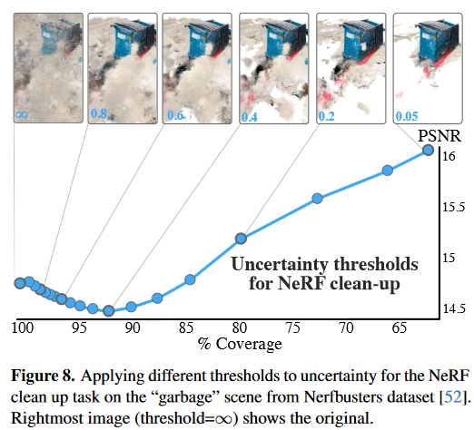
图 8. 对来自 Nerfbusters 数据集 [52] 的“garbage”场景的 NeRF 清理任务的不确定性应用不同的阈值。最左?边的图像(阈值=无穷大)显示原始图像。
6. Conclusions
We have introduced BayesRays, an algorithm to quantify the uncertainty of any trained Neural Radiance Field without independently of its architecture and without additional training nor access to the original training images. Our algorithm outputs a spatial uncertainty field, which we have shown is meaningfully correlated to the NeRF depth error and can be thresholded for use in applications like NeRF cleanup.
我们引入了 BayesRays,这是一种量化任何经过训练的神经辐射场的不确定性的算法,无需独立于其架构,无需额外的训练,也无需访问原始训练图像。我们的算法输出一个空间不确定性场,我们已经证明它与 NeRF 深度误差有意义相关,并且可以设置阈值以用于 NeRF 清理等应用。
We discretize our spatial deformation field using a uniform grid, which can lead to a high memory cost being incurred in regions of little geometric interest. Future work may significantly improve our performance by considering more complex hierarchical data structures like octrees. Separately, in our algorithm’s derivation, we focus only on the diagonal of H, disregarding (minimal) inter-parametric correlations. Future applications may require their inclusion, possibly through low-rank matrix decompositions [2, 3].
我们使用统一网格离散化空间变形场,这可能会导致几何兴趣不大的区域产生较高的内存成本。未来的工作可能会通过考虑更复杂的分层数据结构(如八叉树)来显着提高我们的性能。另外,在我们算法的推导中,我们仅关注 H 的对角线,忽略(最小)参数间相关性。未来的应用可能需要将它们包含在内,可能通过低秩矩阵分解 [2, 3]。
At a higher level, our algorithm’s stated goal is to capture only the epistemic uncertainty of the NeRF, often present through missing or occluded data. As such, aleatoric uncertainty caused by noise or inconsistencies between views is not captured by our method (see Figure 7). We are optimistic that combining our work with current frameworks for aleatoric quantification like [22, 38] will result in a complete study of all sources of uncertainty in NeRF.
在更高的层面上,我们算法的既定目标是仅捕获 NeRF 的认知不确定性,这些不确定性通常通过丢失或遮挡的数据来呈现。因此,我们的方法无法捕获由噪声或视图之间的不一致引起的任意不确定性(见图 7)。我们乐观地认为,将我们的工作与当前的任意量化框架(如 [22, 38])相结合,将导致对 NeRF 中所有不确定性来源的完整研究。
More broadly, our algorithm is limited to quantifying the uncertainty of NeRFs, and cannot be trivially translated to other frameworks. Nonetheless, we look forward to similar deformation-based Laplace approximations being formulated for more recent spatial representations like 3D Gaussian splatting [18]. As the Deep Learning revolution takes Computer Vision algorithms to new horizons of performance and increasingly critical applications, we hope that works like ours can aid in understanding what our models know and do not know as well as the confidence of their guesses.
更广泛地说,我们的算法仅限于量化 NeRF 的不确定性,不能简单地转换到其他框架。尽管如此,我们仍期待着为三维高斯拼接等更新颖的空间表示法制定类似的基于形变的拉普拉斯近似方法[18]。随着深度学习革命将计算机视觉算法带入新的性能领域和日益重要的应用领域,我们希望像我们这样的工作能帮助理解我们的模型知道什么、不知道什么以及它们的猜测的可信度。
抛砖:
- 方法很好,不需要修改训练过程,可直接根据训练好的nerf结果进行评估,而且在nerfstudio框架下,可以可视化,同时能够交互式去除不确定性较高的区域,赞。
- 思路很好,尤其是从摄影测量中获得启发,在不影响重建精度的情况下查询某点的最大扰动扰动来衡量不确定性这一part。
- 在本地进行了复现,跑通了关于poster数据及nerf-facto方法的不确定性评估。
- 关于方法的迁移,在这上面花了半个月时间,在nerfstudio下成功迁移到了vanilla-nerf,用lego数据进行测试,效果不错。但是在nerfstudio下的neus以及sdfstudio下面的neus-facto的尝试都失败了。具体原因在于,在sdf-based nerf相关测试时,对rgb求和并反向传播后,变形点的梯度仍然为none,然后就走不下去了。希望有大佬能够解决这个问题,有可能是模型固有问题,也有可能是代码需要精修。希望有大佬能够进行实现,迁移到sdfstudio下去对sdf-based nerf进行评估。
- 感觉sdf-based nerf急需一个通用不确定性评估方法了,最好也是这种事后框架,看到的大多数论文包括此文,都只对nerf方法进行不确定性评估。sdf相关方法被冷落在一旁。少数提及sdf不确定的也都是不开源的,失望。
启发式算法可以这样定义:一个基于直观或经验构造的算法,在可接受的花费(指计算时间和空间)下给出待解决组合优化问题每一个实例的一个可行解,该可行解与最优解的偏离程度一般不能被预计。 ↩︎
Note this is analogous to the condition number of near/far-field triangulation from photogrammetry that was discussed in Section 1.请注意,这类似于第 1 节中讨论的摄影测量中的近/远场三角测量的条件数。 ↩︎ ↩︎
